Lecture#
Prerequisites#
Ensure you have followed the simulation instructions and have everything set up before running any code in this lecture.
Before You Start
Do a
git pull(native installation only).Recompile Lecture 11 packages.
Source
.bashrc.Check that ROBOT_MODEL is set to rosbot:
echo $ROBOT_MODEL
Pose#
A pose describes the position and orientation of an object in 3D space. Understanding how to represent orientation is fundamental to robotics: every transform, every sensor reading, and every control command depends on it.
Position: where the object is located (a 3D vector \([x, y, z]\)).
Orientation: how the object is rotated or tilted relative to a reference frame.
Note
ROS 2 messages represent pose as geometry_msgs/msg/Pose which
stores position as a Point and orientation as a Quaternion.
Position#
The position of an object is described by a 3D vector:
\(x\): displacement along the forward axis.
\(y\): displacement along the left axis.
\(z\): displacement along the up axis.
Note
Position is unambiguous: three numbers, three axes, one convention. Orientation is far more subtle.
Orientation#
Before publishing transforms, we need to understand how orientations are represented. Orientation can be represented in several ways:
Euler angles (roll, pitch, yaw)
Quaternions
Rotation matrices
Axis-angle representation
Euler Angles
Euler angles (Leonhard Euler) are a set of three angles that describe the orientation of a rigid body with respect to a fixed coordinate system.
Three Angles: Euler angles use three sequential rotations to achieve any desired 3D orientation. These rotations are performed about the axes of a coordinate system.
Different Conventions: There is not one single definition of Euler angles. The most common type in robotics is Tait-Bryan angles (Cardan angles) (e.g., x-y-z, y-z-x) where all three rotations are about different axes. Also known as roll, pitch, and yaw.
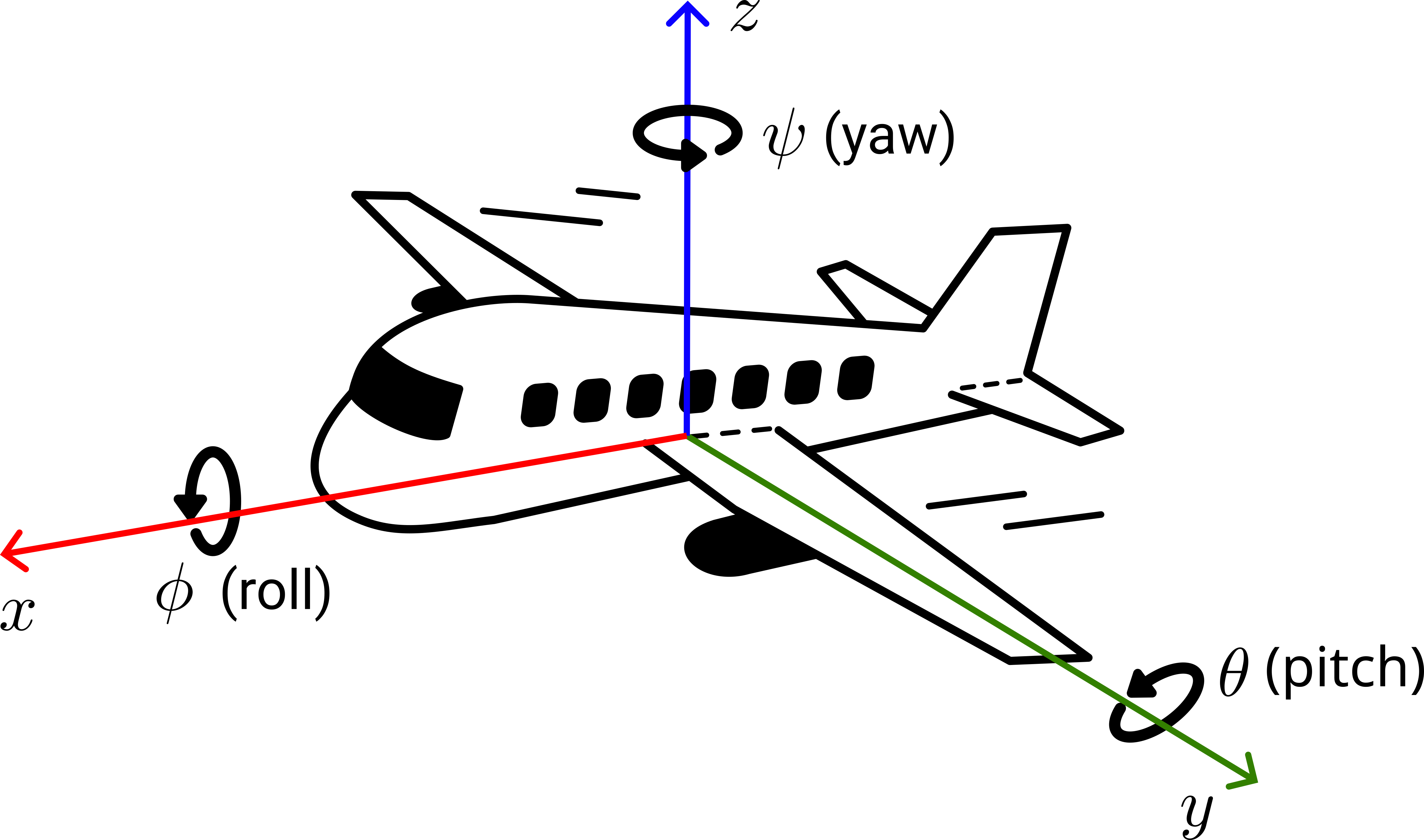
Fig. 86 Rotation about the \(x\)-, \(y\)-, and \(z\)-axis.#
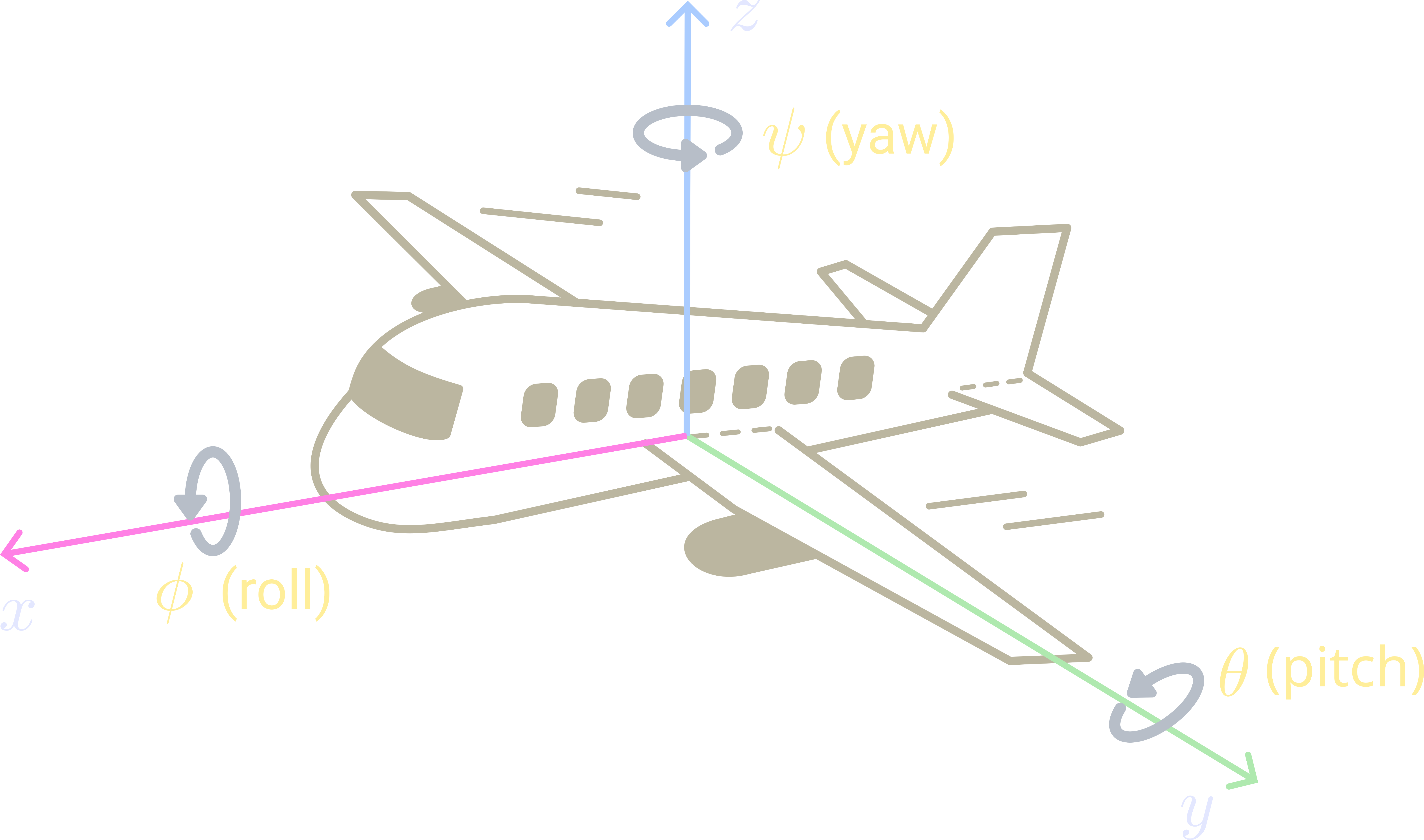
Fig. 87 Rotation about the \(x\)-, \(y\)-, and \(z\)-axis.#
Roll (\(\phi\)): rotation about the \(x\)-axis (tilting side to side).
Pitch (\(\theta\)): rotation about the \(y\)-axis (tilting forward/backward).
Yaw (\(\psi\)): rotation about the \(z\)-axis (turning left/right).
The Gimbal Lock Problem
Despite their intuitiveness, Euler angles suffer from a critical flaw called gimbal lock: when two rotation axes align (e.g., pitch reaches \(\pm 90°\)), one degree of freedom is lost and certain orientations become unreachable through smooth rotation.
Why this matters in robotics:
A robot arm approaching certain orientations may experience erratic behavior as the controller tries to compensate for the singularity.
Interpolating between two orientations using Euler angles can produce unexpected paths through gimbal-lock configurations.
Small orientation changes near the singularity require enormous changes in the angle values, causing numerical instability.
Note
This is why ROS 2, game engines, and aerospace systems use quaternions for representing orientations. Quaternions are singularity-free. See Appendix A: Gimbal Lock for the mathematical proof.
Quaternions#
The Intuition
Before the formal math, here is the key idea:
Note
A quaternion encodes a rotation as an axis (which direction to rotate around) and an angle (how far to rotate). Think of it as pointing your thumb along an axis and curling your fingers by some angle.
Given a unit axis \(\mathbf{u} = (u_x, u_y, u_z)\) and a rotation angle \(\theta\):
Reading a quaternion:
The scalar part \(w\) tells you how much rotation: \(w = 1\) means no rotation; \(w = 0\) means a \(180°\) rotation.
The vector part \((x, y, z)\) tells you which direction the rotation axis points.
The vector’s magnitude encodes the rotation amount (along with \(w\)).
Formal Definition
A quaternion (William Rowan Hamilton, 1843) extends complex numbers to four dimensions. It consists of four components:
Or more compactly: \(q = (w, x, y, z)\).
\(w\) is the scalar part (real number).
\(x\), \(y\), \(z\) are the components of the vector part.
\(i\), \(j\), \(k\) are the imaginary basis units, satisfying: \(i^2 = j^2 = k^2 = ijk = -1\).
Unit Quaternions
For representing rotations, we use unit quaternions (magnitude equal to 1):
A quaternion \(q = w + xi + yj + zk\) is just a point in 4D space. Most of those points have nothing to do with rotations. The constraint \(|q| = 1\) restricts you to the surface of a 4D unit sphere, called \(S^3\). It turns out that this particular surface has exactly the right algebraic structure to encode every possible 3D rotation, with no redundancy except the unavoidable double cover (\(q\) and \(-q\) map to the same rotation).
Warning
Double cover: \(q\) and \(-q\) represent the same rotation. For example, \((w, x, y, z) = (0.707, 0.707, 0, 0)\) and \((-0.707, -0.707, 0, 0)\) both encode a \(90°\) rotation about the \(x\)-axis. This can cause sign-flip artifacts when interpolating or comparing quaternions.
Common Quaternion Values
Building intuition through examples:
Rotation |
Quaternion \((w,x,y,z)\) |
Notes |
|---|---|---|
No rotation (identity) |
\((1,\; 0,\; 0,\; 0)\) |
\(w=1\), no axis needed |
\(90°\) about Z (yaw left) |
\((0.707,\; 0,\; 0,\; 0.707)\) |
Only \(z\) component |
\(180°\) about Z (face backward) |
\((0,\; 0,\; 0,\; 1)\) |
\(w=0 \Rightarrow\) half turn |
\(90°\) about X (roll right) |
\((0.707,\; 0.707,\; 0,\; 0)\) |
Only \(x\) component |
\(45°\) about Y (pitch up) |
\((0.924,\; 0,\; 0.383,\; 0)\) |
Small angle \(\Rightarrow w\) near 1 |
Note
Notice the pattern: the vector part \((x,y,z)\) points along the rotation axis, and \(w\) closer to 1 means a smaller rotation angle. When rotating about a single world axis (X, Y, or Z), only one vector component is non-zero. For an arbitrary axis, all three can be non-zero simultaneously.
Axis-Angle to Quaternion Conversion
Given a unit axis \(\mathbf{u} = (u_x, u_y, u_z)\) and rotation angle \(\theta\) (in radians):
The scalar part is \(w = \cos(\theta/2)\) and the vector part is:
Note
Why \(\theta/2\) and not \(\theta\)? This half-angle encoding is what makes quaternion multiplication correctly compose rotations. It also ensures \(q\) and \(-q\) map to the same rotation (the double cover property).
Rotating Vectors with Quaternions
To rotate a 3D vector \(\mathbf{v}\) using a unit quaternion \(q\), represent the vector as a “pure” quaternion (with a scalar part of zero): \(p = 0 + v_x\, i + v_y\, j + v_z\, k\). The rotated vector \(\mathbf{v}'\) (as a pure quaternion \(p'\)) is:
For a unit quaternion, the inverse is simply its conjugate: \(q^{-1} = w - x\,i - y\,j - z\,k\).
Composition of Rotations
Multiple rotations can be combined by multiplying their quaternions.
\(q_1\) represents a rotation, \(q_2\) represents another rotation.
\(q_{\text{combined}} = q_2 \otimes q_1\) represents the combined rotation (\(q_1\) applied first, then \(q_2\)).
Warning
Quaternion multiplication is not commutative: \(q_1 \otimes q_2 \neq q_2 \otimes q_1\). Choosing the wrong order will produce an incorrect result!
Quaternion Multiplication Order
The order of quaternion multiplication depends on the frame of reference for the rotation.
Frame |
Description |
Formula |
|---|---|---|
World/Fixed |
Rotate about a global axis |
\(O_{\text{final}} = O_{\text{rot}} \otimes O_{\text{init}}\) |
Body/Local |
Rotate about object’s own axis |
\(O_{\text{final}} = O_{\text{init}} \otimes O_{\text{rot}}\) |
World Frame Rotation
Axis is fixed in space.
“Rotate about the global x-axis.”
Independent of object’s current orientation.
Body Frame Rotation
Axis moves with the object.
“Roll the aircraft” (about its nose-to-tail axis).
Depends on object’s current orientation.
Note
In aviation and robotics, body-frame rotations are more common. A pilot’s roll, pitch, and yaw commands rotate about the aircraft’s own axes, not the world axes.
Exercise: Quaternion from Axis-Angle
Calculate the rotation, expressed as a quaternion, resulting from a rotation of \(\alpha = \frac{\pi}{2}\) radians about the \(x\)-axis.
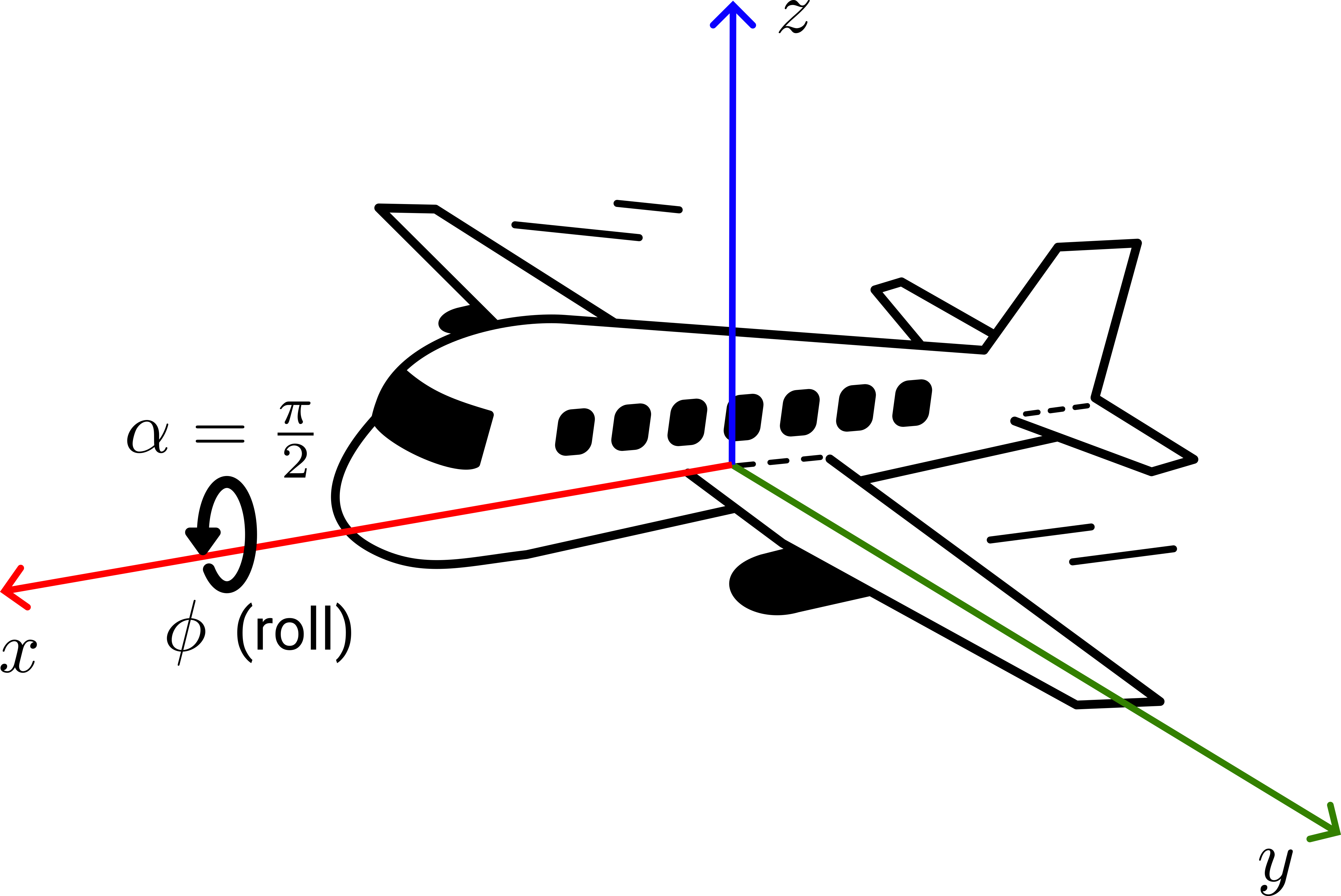
Fig. 88 A rotation of \(\alpha = \frac{\pi}{2}\) radians about the \(x\)-axis.#
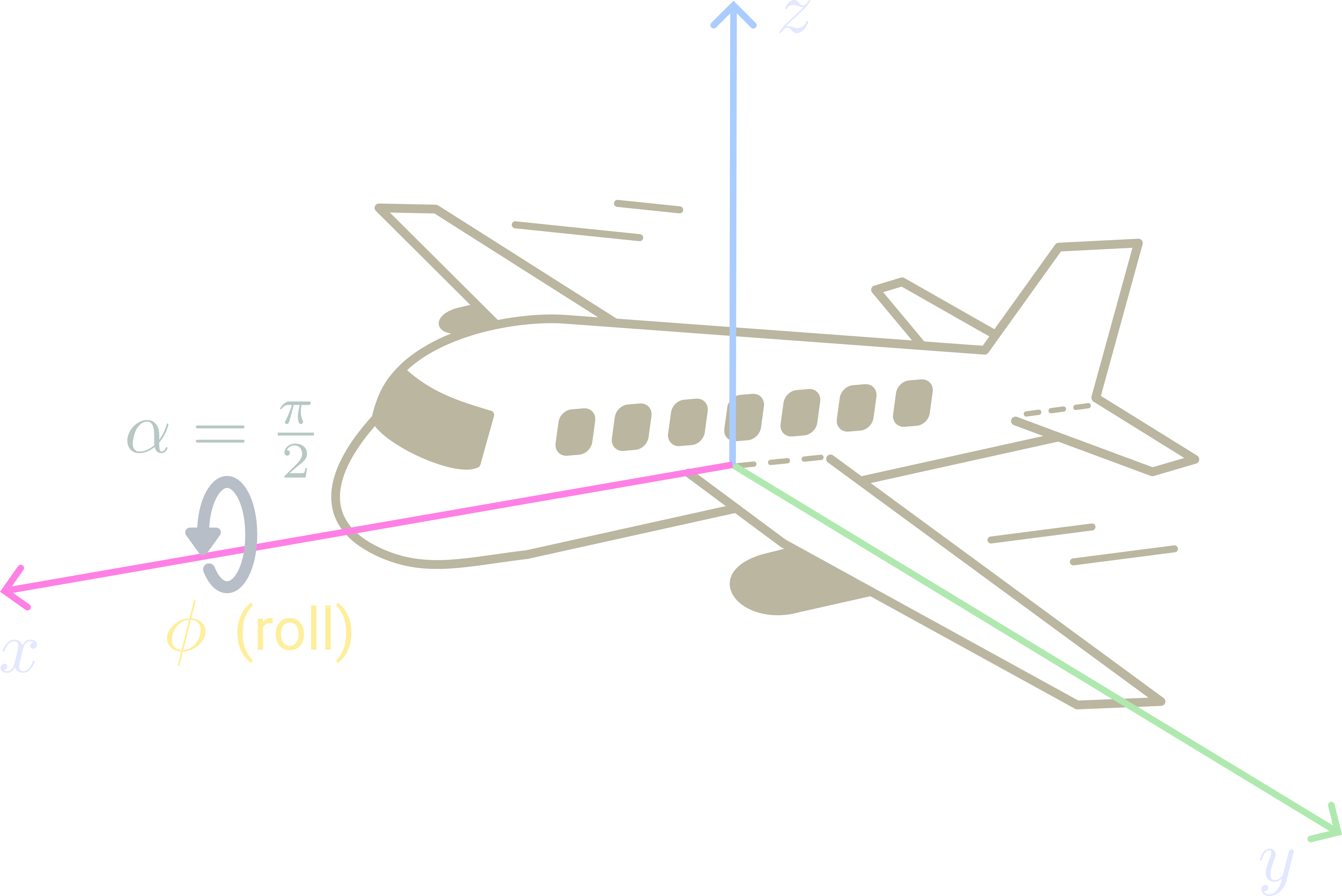
Fig. 89 A rotation of \(\alpha = \frac{\pi}{2}\) radians about the \(x\)-axis.#
Identify the axis and angle
The rotation is about the \(x\)-axis, so \(\mathbf{u} = (1, 0, 0)\) and \(\alpha = \frac{\pi}{2}\).
Verify the axis is a unit vector
The axis-angle formula requires \(\|\mathbf{u}\| = 1\):
\[\|\mathbf{u}\| = \sqrt{u_x^2 + u_y^2 + u_z^2} = \sqrt{1^2 + 0^2 + 0^2} = 1 \quad \checkmark\]Apply the axis-angle formula
\[q = \cos\!\left(\frac{\alpha}{2}\right) + \sin\!\left(\frac{\alpha}{2}\right)(u_x\, i + u_y\, j + u_z\, k) = \cos\!\left(\frac{\pi}{4}\right) + \sin\!\left(\frac{\pi}{4}\right)(1 \cdot i + 0 \cdot j + 0 \cdot k)\]Compute each component
\(w = \cos\!\left(\frac{\alpha}{2}\right) = \cos\!\left(\frac{\pi}{4}\right) = \frac{\sqrt{2}}{2} \approx 0.707\)
\(x = \sin\!\left(\frac{\alpha}{2}\right) \times u_x = \sin\!\left(\frac{\pi}{4}\right) \times 1 = \frac{\sqrt{2}}{2} \approx 0.707\)
\(y = \sin\!\left(\frac{\alpha}{2}\right) \times u_y = \sin\!\left(\frac{\pi}{4}\right) \times 0 = 0.0\)
\(z = \sin\!\left(\frac{\alpha}{2}\right) \times u_z = \sin\!\left(\frac{\pi}{4}\right) \times 0 = 0.0\)
Resulting quaternion
\[q = (w, x, y, z) = \left(\frac{\sqrt{2}}{2},\, \frac{\sqrt{2}}{2},\, 0,\, 0\right) \approx (0.707,\, 0.707,\, 0.0,\, 0.0)\]Verify: Does this match the table from earlier? A \(90°\) rotation about \(x\) should have \(w \approx 0.707\) and only the \(x\) component non-zero.
Note
Remember the double cover: \((-0.707, -0.707, 0, 0)\) represents the same rotation.
Mobile Robot Control#
This course uses two Husarion ROSbot platforms, both supported by the same rosbot_ros ROS 2 driver.

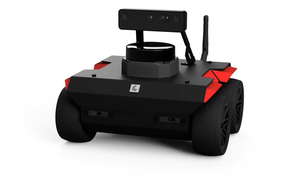
Drive: differential (4-wheel)
SBC: Raspberry Pi 5
Sensors: RPLiDAR, Luxonis OAK-D, IMU
ROS 2 model:
rosbot
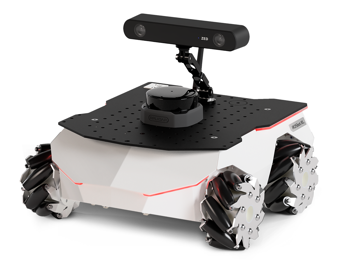

Drive: differential or mecanum (4-wheel)
SBC: Raspberry Pi 5 / Jetson Orin / NUC
Sensors: LiDAR, RGB-D camera, IMU
ROS 2 model:
rosbot_xl
ros2 launch rosbot_gazebo husarion_world.launch.py
Gazebo#
Gazebo is an open-source 3D robot simulator. It provides a physics engine, sensor simulation, and a world environment so that ROS 2 nodes can be developed and tested without access to physical hardware.
Note
This course uses Gazebo Harmonic, the version paired with ROS 2 Jazzy.
Gazebo simulates the physical world so that ROS 2 nodes behave identically whether they run against real hardware or a simulation.
Physics engine: models rigid body dynamics, collisions, friction, and inertia.
Sensor simulation: generates realistic LiDAR scans, camera images, and IMU readings with configurable noise.
ROS 2 bridge: the
ros_gz_bridgepackage forwards Gazebo topics to ROS 2 topics, making the simulation transparent to your nodes.World files: environments are defined in SDF format and can range from an empty plane to a full indoor building.
Note
From your node’s perspective, a simulated ROSbot and a real ROSbot look identical: the same topics, the same transforms, the same message types. The only difference is where the data originates.
RViz2#
RViz2 is the standard ROS 2 visualization tool. It does not simulate anything: it subscribes to ROS 2 topics and renders the data in 3D, giving you a live view of what the robot perceives and where it thinks it is.
RViz2 is a passive subscriber: it reads data from running nodes and renders it visually. It never publishes commands or modifies the robot’s state.
Every visual element in RViz2 is called a display.
Each display subscribes to one or more ROS 2 topics and renders the data in the 3D viewport.
Displays can be added, removed, and configured at runtime without restarting RViz2.
The Fixed Frame setting determines which coordinate frame the scene is rendered relative to. All other frames are drawn relative to it.
Note
RViz2 configuration can be saved to a .rviz file and loaded at
startup:
rviz2 -d path/to/config.rviz
Key Displays for This Course
Display |
Topic |
What it shows |
|---|---|---|
TF |
|
All coordinate frames as colored axes. |
RobotModel |
|
The robot’s URDF mesh rendered in 3D. |
Odometry |
|
Robot pose history as a trail of arrows. |
LaserScan |
|
LiDAR point cloud as colored dots. |
Image |
|
RGB camera feed in a 2D overlay panel. |
PointCloud2 |
|
Stereo depth point cloud in 3D. |
Imu |
|
IMU orientation and acceleration arrows. |
Axes |
(manual) |
A single coordinate frame for reference. |
Note
Set Fixed Frame to odom when visualizing robot motion, and to
map when working with a known map. If RViz2 shows a grey scene
with no data, the Fixed Frame is likely set to a frame that does not
yet exist in the TF tree.
Differential Drive Model#
The differential drive model relates wheel velocities to the robot’s linear and angular velocity. Understanding this model is essential before designing a controller.
Linear Velocity (\(v\)): Rate of change of position along the robot’s heading direction.
Angular Velocity (\(\omega\)): Rate of change of orientation (heading angle).
Note
Sign Convention: \(v > 0\) moves forward, \(v < 0\) moves backward. \(\omega > 0\) turns counterclockwise (left), \(\omega < 0\) turns clockwise (right). Combining both produces curved trajectories.
Kinematics
Let \(v_L\) and \(v_R\) be the left and right wheel speeds, \(L\) the wheel separation, and \(r\) the wheel radius.
From wheel speeds to body velocities:
From body velocities to wheel speeds:
\(v\): linear velocity (m/s), sent as
twist.linear.x\(\omega\): angular velocity (rad/s), sent as
twist.angular.zOnly
linear.xandangular.zare used for ground robots.Other components (
linear.y,angular.x,angular.y) are set to zero.
Note
Although both ROSbots have four wheels, the two left wheels are driven together and the two right wheels are driven together. The kinematics therefore reduce to the standard two-variable differential drive model above.
The /cmd_vel Topic
Velocity commands are sent to the robot by publishing on /cmd_vel.
In ROS 2 Jazzy the expected message type is
geometry_msgs/msg/TwistStamped.
std_msgs/Header header
    builtin_interfaces/Time stamp
        int32 sec
        uint32 nanosec
    string frame_id
Twist twist
    Vector3  linear
        float64 x
        float64 y
        float64 z
    Vector3  angular
        float64 x
        float64 y
        float64 z
For a differential drive robot, only
twist.linear.xandtwist.angular.zcarry meaningful values.The
header.stampshould be set to the current time so controllers can reject stale commands.The
header.frame_ididentifies the frame the twist is expressed in (usuallybase_link).
Velocity Command Reference
|
|
Motion |
|---|---|---|
\(> 0\) |
\(0\) |
Straight forward |
\(< 0\) |
\(0\) |
Straight backward |
\(0\) |
\(> 0\) |
Rotate left (counterclockwise) |
\(0\) |
\(< 0\) |
Rotate right (clockwise) |
\(> 0\) |
\(> 0\) |
Curve forward to the left |
\(> 0\) |
\(< 0\) |
Curve forward to the right |
\(< 0\) |
\(> 0\) |
Curve backward to the right |
\(< 0\) |
\(< 0\) |
Curve backward to the left |
Note
All other fields of geometry_msgs/Twist (linear.y,
linear.z, angular.x, angular.y) are always set to zero
for a ground differential drive robot.
Odometry#
Odometry is the process of estimating a robot’s current pose (position and orientation) by integrating motion data over time. It answers the question: where is the robot now, given where it started and how it has moved?
As the robot moves, its wheels rotate. Each wheel is equipped with a quadrature encoder that counts the number of pulses per revolution. By knowing the wheel radius and the number of pulses, the firmware computes how far each wheel has traveled.
From those distances, the differential drive kinematics equations compute:
How far the robot has moved forward (\(\Delta s\)).
How much the robot has turned (\(\Delta \psi\)).
These incremental changes are integrated over time to produce the
robot’s estimated pose \((x, y, \psi)\) in the odom frame:
Warning
Odometry drifts over time. Small errors in each step accumulate,
so the estimated pose diverges from the true pose. This is why the
ROSbot fuses wheel odometry with IMU data via an Extended Kalman
Filter to produce odometry/filtered.
The nav_msgs/msg/Odometry Message
The nav_msgs/msg/Odometry message bundles everything a consumer
needs to know about the robot’s estimated motion:
header.frame_id: the frame in which the pose is expressed (typically
odom).child_frame_id: the frame being described (typically
base_link).pose.pose: the estimated position \((x, y, z)\) and orientation (quaternion).
pose.covariance: a \(6 \times 6\) covariance matrix encoding the uncertainty in the pose estimate.
twist.twist: the robot’s estimated linear and angular velocity in the
base_linkframe.twist.covariance: uncertainty in the velocity estimate.
Note
The ROSbot publishes two odometry topics: odometry/wheels
contains the raw wheel-encoder estimate, and odometry/filtered
contains the EKF-fused estimate that also incorporates IMU data.
Always use odometry/filtered for control.
Odometry in RViz2
When you add an Odometry display in RViz2 and point it at
odometry/filtered, you will see a red arrow appear at the
robot’s estimated position.
Reading the Arrow
Arrow origin: the robot’s estimated \((x, y)\) position in the
odomframe.Arrow direction: the robot’s estimated heading \(\psi\) (yaw). The arrow points in the direction the robot is facing.
Arrow length: proportional to the robot’s current linear speed \(v\). A stationary robot shows a very short arrow; a fast-moving robot shows a long one.
Keep last N: RViz2 can retain the last \(N\) arrows, leaving a trail that shows the robot’s path over time.
Note
If the arrow does not appear, check that the Fixed Frame is set
to odom and that the odometry/filtered topic is being
published. You can verify with:
ros2 topic echo odometry/filtered --once
Demonstration
Review
random_mover_demo.pyfromrobot_control_demo.Start the environment:
ros2 launch rosbot_gazebo empty_world.launch.pyRandomly move the robot:
ros2 run robot_control_demo random_mover
Proportional Controller#
A proportional (P) controller produces a command proportional to the error between the desired state and the current state. It is the simplest feedback controller and a natural first step toward more sophisticated designs.
The P Controller Law
\(e\) is the error: the difference between the goal and the current state.
\(K_p\) is the proportional gain: a tuning constant that scales the response.
\(u\) is the control output: the velocity command sent to the robot.
Error |
Meaning |
Command |
|---|---|---|
Distance to goal (\(\rho\)) |
How far away is the goal? |
Linear velocity \(v\) |
Heading error (\(\alpha\)) |
How misaligned is the robot? |
Angular velocity \(\omega\) |
Mobile Robot Application#
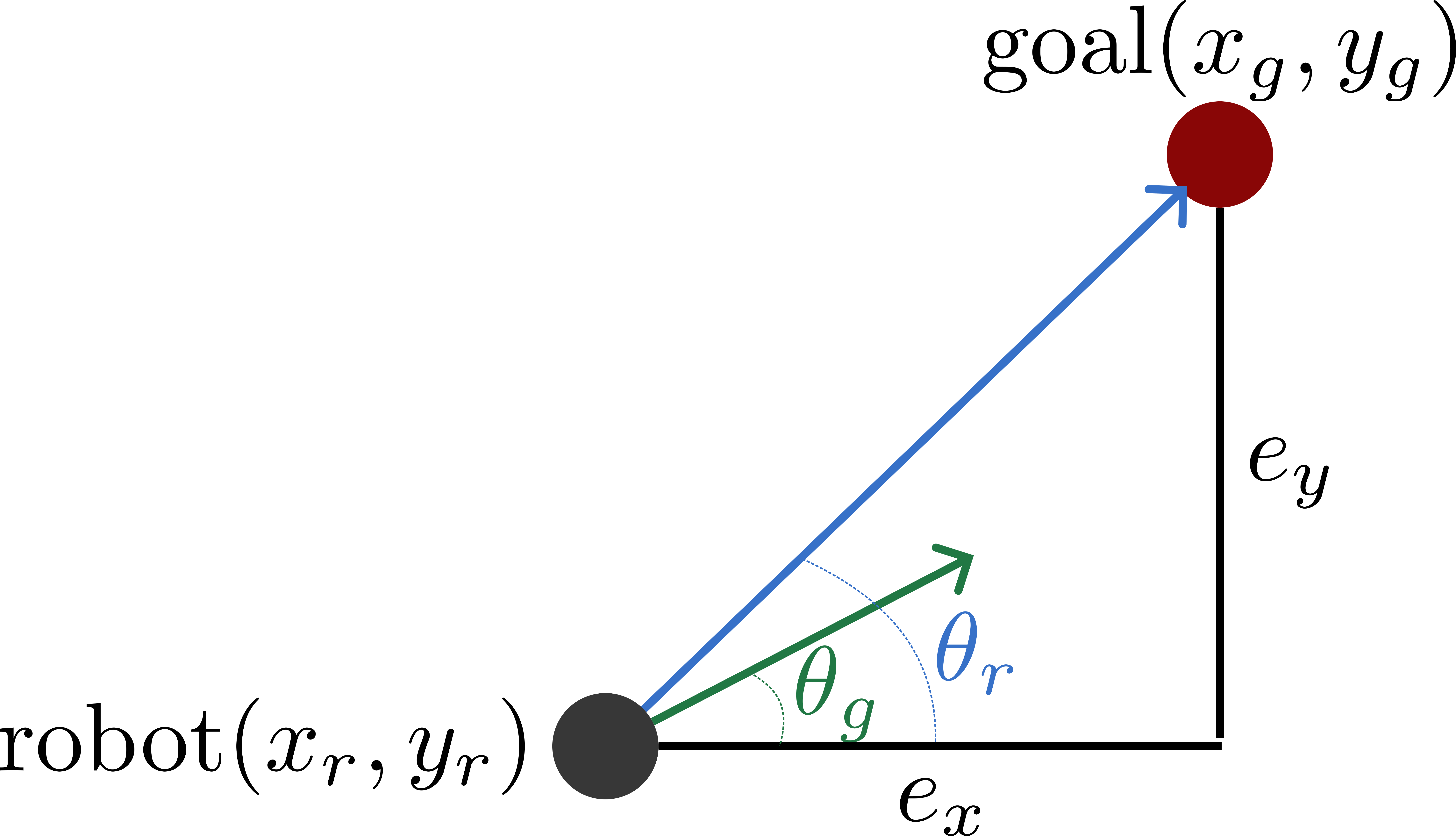
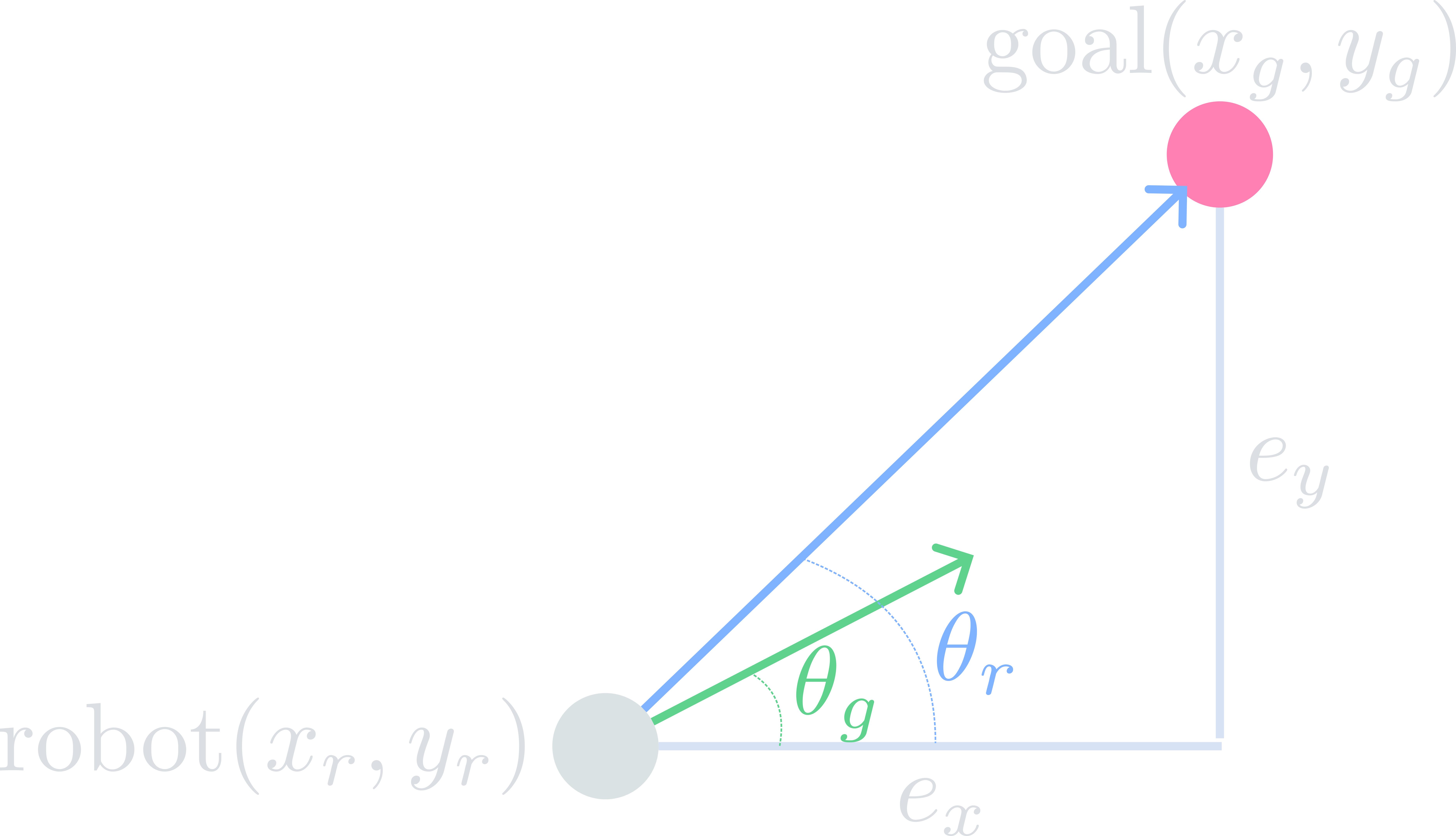
where \(\theta_g = \text{atan2}(e_y, e_x)\).
Note
As the robot approaches the goal, errors decrease, velocities decrease, and the robot stops at the goal.
Example: Reaching a Goal 5 m Away
Reach the goal, which is 5 m from the current position of the robot (straight line).
We will assume a value for the proportional gain, e.g., \(K_{pv}=0.5\,\text{s}^{-1}\). The units ensure that when multiplied by distance in meters, we get velocity in m/s.
Step-by-Step Example: Reaching a Goal 5 m Away
Assume \(K_{pv} = 0.5\,\text{s}^{-1}\).
At \(t_0\): error \(= 5\) m \(\rightarrow\) \(u(t) = 0.5 \times 5 = 2.5\) m/s \(\rightarrow\) distance traveled \(\approx 2.4\) m
At \(t_1\): error \(= 2.6\) m \(\rightarrow\) \(u(t) = 0.5 \times 2.6 = 1.3\) m/s \(\rightarrow\) distance traveled \(\approx 3.6\) m
At \(t_2\): error \(= 1.4\) m \(\rightarrow\) \(u(t) = 0.5 \times 1.4 = 0.7\) m/s \(\rightarrow\) distance traveled \(\approx 4.3\) m
… continues until the error falls below the tolerance.
As the robot approaches the goal, errors decrease, velocities decrease, and the robot stops at the goal. This is the essence of proportional control.
Limitations of a Pure P Controller
Steady-state error: the robot may stop slightly before the goal if the gain is too low, or oscillate around it if the gain is too high.
No integral term: persistent disturbances (e.g., wheel slip, uneven terrain) accumulate and are never corrected.
No derivative term: the controller does not anticipate rapid changes in error, which can cause overshoot.
Heading-only correction: this design corrects heading and distance independently. For curved paths, a PID or pure pursuit controller is more appropriate.
Note
A P controller is an excellent starting point for learning closed-loop control. PID and model-predictive controllers build directly on the same error-signal concept.
Proportional Control for Angle Reaching
The same proportional control reasoning applies to reaching a certain orientation (heading angle).
Instead of distance error, use angular error: \(e_\psi = \psi_{\text{goal}} - \psi_{\text{robot}}\)
The control output is angular velocity: \(\omega = K_{p\omega} \cdot e_\psi\)
As the heading error decreases, the angular velocity decreases, and the robot settles at the desired orientation.
Note
In the full go-to-goal controller, both linear and angular proportional control work simultaneously: the robot adjusts its heading toward the goal while moving forward, resulting in a smooth curved trajectory.
Demonstration
Review
p_controller_demo.pyfromrobot_control_demo.Start the environment:
ros2 launch rosbot_gazebo empty_world.launch.pyReach a goal:
ros2 launch robot_control_demo p_controller.launch.pyObserve in RViz2: add an Odometry display and watch the robot’s path.
Tip
Experiment: Increase k_rho to 1.0. What changes? Now decrease
it to 0.1. What happens near the goal? What value gives the best
trade-off between speed and precision?
Coordinate Frames#
A coordinate frame (or reference frame) is a named origin with three orthogonal axes used to express positions and orientations. In robotics, multiple frames are needed simultaneously: the world has its own frame, the robot body has its own frame, and each sensor has its own frame.
Why Multiple Frames#
A LiDAR mounted on a robot reports obstacle distances relative to itself, not relative to the world.
A camera reports pixel coordinates that must be related to the robot body and then to the world to be useful.
A goal pose provided to a planner is in the world frame; the robot must know its own pose in that frame to compute the required motion.
Note
Without a consistent way to track how all these frames relate to each other, a multi-sensor robot cannot function. TF2 provides this bookkeeping automatically.
Right-Hand Rule#
ROS 2 uses the right-hand rule for coordinate frames:
X axis: forward
Y axis: left
Z axis: up
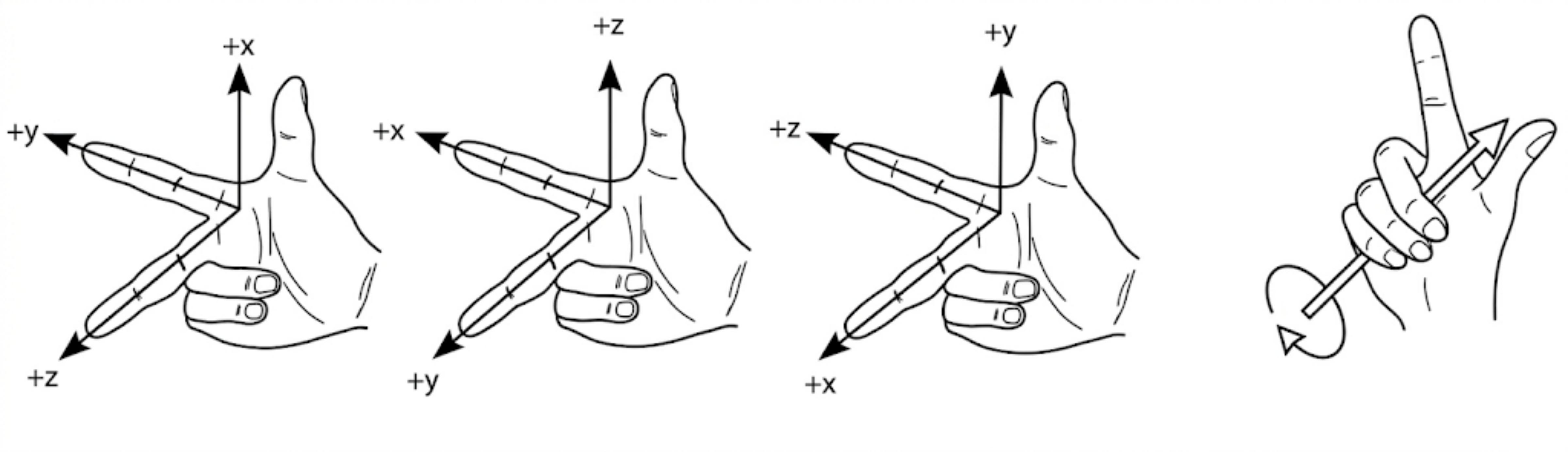
Fig. 90 ROS uses the right-hand rule.#
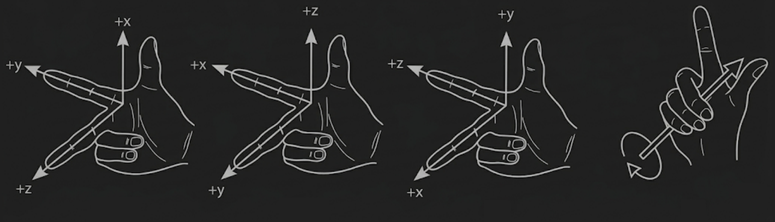
Fig. 91 ROS uses the right-hand rule.#
Note
In ROS, the axes are color coded: \(x\) is red, \(y\) is green, and \(z\) is blue.
Why Are Frames Important?
Imagine telling a robot to pick up an object. You might know the object’s location relative to a camera. However, the robot’s arm controller needs to know where to move its joints relative to its own base. This is where frames come in.
Frames provide a consistent way to represent and reason about spatial relationships between different entities in the robot’s environment.
Sensor Fusion: Data from different sensors (camera, LiDAR, IMU) are expressed in their own sensor-specific frames. To combine and interpret this data, we need to transform it into a common frame of reference.
Navigation: For a robot to navigate effectively, it needs to know its pose (position and orientation) relative to a global map frame.
Manipulation: Precise control of robot arms requires understanding the transformations between the robot’s base frame, the end-effector frame, and the object frame.
Standard Mobile Robot Frames (REP 105)#
Frame |
Description |
|---|---|
|
Global inertial frame. Fixed. Used when a long-term, drift-free reference is required. |
|
The robot’s best estimate of its global position. May jump when the localization estimate is corrected (e.g., loop closure). |
|
Locally consistent, drift-prone frame computed from wheel odometry or IMU. Never jumps; drifts over time. |
|
Rigidly attached to the robot body. Typically at the geometric center of the base, at ground level. |
|
Projection of |
Sensor frames |
Attached to each sensor (e.g., |
Transforms#
A transform describes how to express the pose of one coordinate frame relative to another. It answers the question: if I know a point’s coordinates in frame A, what are its coordinates in frame B?
Every transform between two frames in 3D space consists of two components:
Translation: a 3D vector \(\mathbf{t} = (t_x, t_y, t_z)\) describing how far and in which direction the origin of frame \(B\) is displaced from the origin of frame \(A\).
Rotation: a description of how frame \(B\)’s axes are oriented relative to frame \(A\)’s axes (expressed as a quaternion in ROS 2).
In ROS 2, a transform between two frames is represented by the
geometry_msgs/TransformStamped message:
ros2 interface show geometry_msgs/msg/TransformStamped
# This expresses a transform from coordinate frame header.frame_id
# to the coordinate frame child_frame_id at the time of header.stamp
#
# This message is mostly used by the tf2 package.
# See its documentation for more information.
#
# The child_frame_id is necessary in addition to the frame_id
# in the Header to communicate the full reference for the transform
# in a self contained message.

# The frame id in the header is used as the reference frame of this transform.
std_msgs/Header header
    builtin_interfaces/Time stamp
        int32 sec
        uint32 nanosec
    string frame_id

# The frame id of the child frame to which this transform points.
string child_frame_id

# Translation and rotation in 3-dimensions of child_frame_id from header.frame_id.
Transform transform
    Vector3 translation
        float64 x
        float64 y
        float64 z
    Quaternion rotation
        float64 x 0
        float64 y 0
        float64 z 0
        float64 w 1
A coordinate frame in isolation has no spatial meaning: knowing that a frame exists tells you nothing about where it is or how it is oriented unless you also know its transform relative to some other frame.
The only exception is the root frame:
Every transform tree has exactly one root, typically
world.The root frame is defined by convention as the fixed global reference; it has no parent and therefore requires no transform.
Every other frame in the system must have a transform connecting it to its parent, and through that parent, ultimately to
world.
A transform \(T^{A}_{B}\) expresses frame \(B\) relative to frame \(A\). Direction matters.
\(T^{A}_{B}\) tells you where \(B\) is when you are standing in \(A\).
\(T^{B}_{A}\) is the inverse transform: it tells you where \(A\) is when you are standing in \(B\).
Inverting a transform reverses both the rotation and the translation: you cannot simply negate the translation vector.
Given a point \(\mathbf{p}_B\) expressed in frame \(B\), the same point expressed in frame \(A\) is:
where \(R^{A}_{B}\) is the \(3 \times 3\) rotation matrix that rotates vectors from frame \(B\) into frame \(A\), and \(\mathbf{t}^{A}_{B}\) is the translation vector of the origin of \(B\) expressed in \(A\).
Transforms can be chained: if you know \(T^{A}_{B}\) and \(T^{B}_{C}\), you can compute \(T^{A}_{C}\) directly using \(4 \times 4\) homogeneous transformation matrices:
The inner indices cancel, which is a useful consistency check: \(B\) appears as a subscript on the left and a superscript on the right, and drops out of the result.
TF2#
TF2 (Transform Library, version 2) is the ROS 2 library responsible for tracking coordinate frames over time. Rather than requiring every node to manually compute and share transforms, TF2 provides a shared, system-wide bookkeeping service that any node can publish to or query from.
What TF2 Does
Stores all transforms broadcast by any node in a time-stamped buffer.
Answers queries of the form: “what is the transform from frame \(A\) to frame \(B\) at time \(t\)?”
Interpolates between stored transforms to give the best estimate at any requested timestamp.
Chains intermediate transforms automatically so callers never need to compose them by hand.
Note
TF2 is not a node you run explicitly. It is a library: any node that
creates a TransformBroadcaster or TransformListener is
participating in the TF2 system automatically.
The TF2 Transform Tree
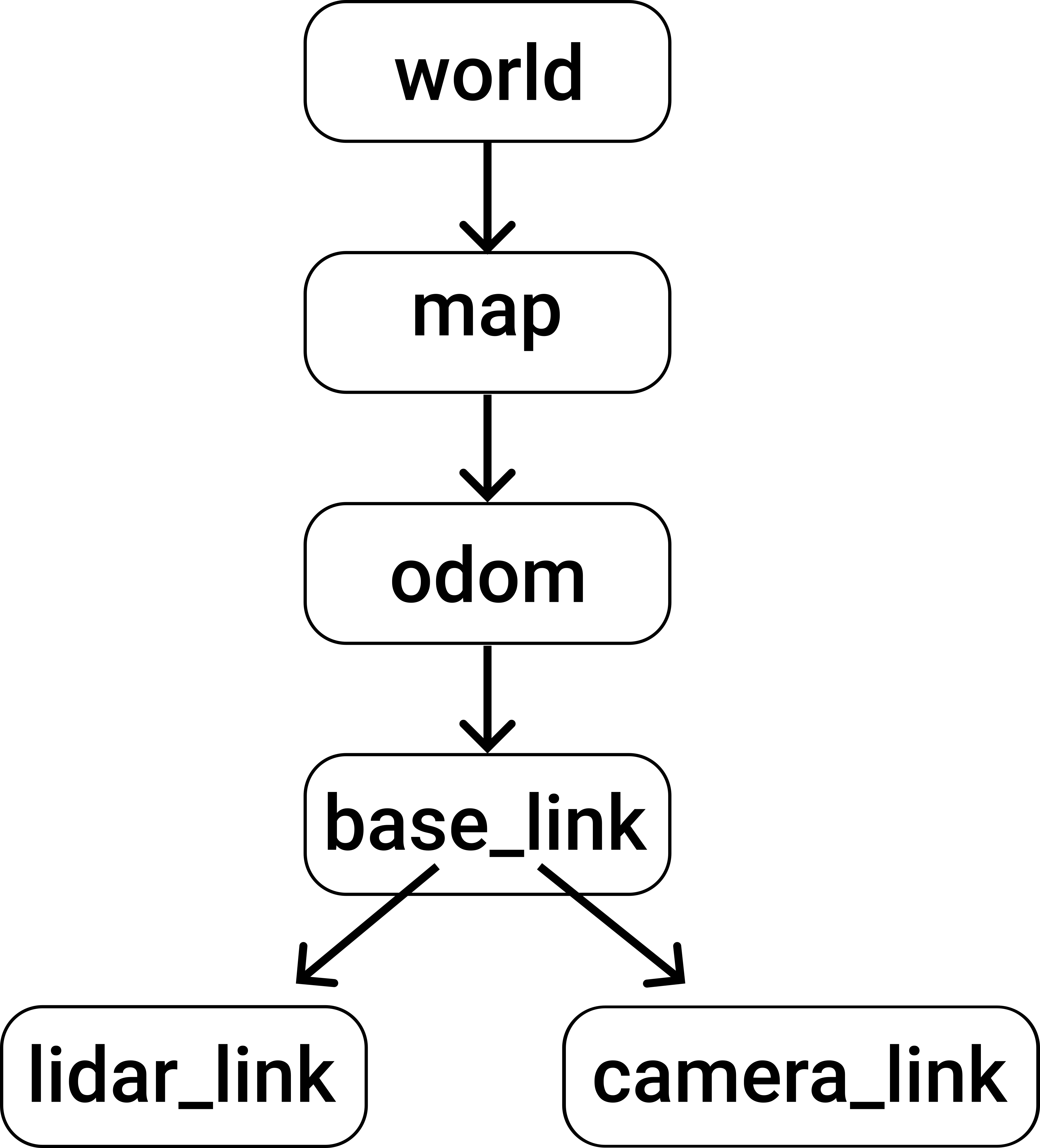
Fig. 92 TF2 transform tree.#
Fig. 93 TF2 transform tree.#
TF2 maintains a tree of transforms, where each edge represents the transform from a parent frame to a child frame.
The tree is directed: every child has exactly one parent, but a parent may have many children.
To find the transform between any two frames, TF2 traverses the tree from one frame up to the common ancestor and back down to the other.
TF2 CLI Tools
ros2 run tf2_tools view_frames
Saves a PDF of the current transform tree to
frames_<timestamp>.pdf.Useful for verifying that all expected frames are connected.
ros2 run tf2_ros tf2_echo <source_frame> <target_frame>
Continuously prints the transform from
source_frametotarget_frame.
ros2 topic echo /tf
ros2 topic echo /tf_static
Raw transform messages published on these two topics by all broadcasters.
/tfreceives dynamic (time-varying) transforms./tf_staticreceives static (time-invariant) transforms, published once and latched.
ros2 run rqt_tf_tree rqt_tf_tree --force-discover
Provides the TF2 tree in a graphical user interface.
Demonstration
Start empty environment:
ros2 launch rosbot_gazebo empty_world.launch.pyTry each CLI tool.
Static Transforms#
A static transform describes the fixed geometric relationship
between two frames that does not change over time, for example the
offset from base_link to a rigidly mounted sensor such as a LiDAR
or camera.
CLI: static_transform_publisher
ROS 2 ships a convenience node for publishing a single static transform from the command line.
ros2 run tf2_ros static_transform_publisher --help
Demonstration
Publish a transform from body_link to lidar_link:
T1:
ros2 launch rosbot_gazebo empty_world.launch.pyT2:
ros2 run tf2_ros static_transform_publisher --x 0.2 --y 0.0 --z 0.15 \
  --frame-id body_link --child-frame-id lidar_link
T3:
ros2 run tf2_ros tf2_echo body_link lidar_linkT4:
ros2 run rqt_tf_tree rqt_tf_tree --force-discover
Note
This is useful for quick debugging. For production, prefer embedding the transform in the robot URDF or broadcasting it from a node.
Scenario: ArUco Marker Detection (Static)
Goal: detect an ArUco marker in a camera image, recover its 3D pose from the 2D corners using the camera intrinsics, and publish that pose once as a static TF from the camera optical frame to a child frame
static_aruco_box.Why static? The marker (and the overhead camera) do not move, so one latched transform on
/tf_staticis enough (no need to re-broadcast every frame).Inputs needed:
the color image (2D pixel corners of the marker),
CameraInfo(intrinsics \(K\) and distortion \(d\)),the known physical marker size (meters).
Approach: PnP (see Appendix B: Perspective-n-Point (PnP)).
Implementation:
static_aruco_detector.pyEnvironment:
ros2 launch rosbot_gazebo aruco_box_camera_world.launch.py
We need image pixels, intrinsics, and a latched static TF publisher.
# Image pixels
self._image_sub = self.create_subscription(
    Image, self._camera_image_topic,
    self._image_callback, qos_profile_sensor_data,
)
# Intrinsics
self._info_sub = self.create_subscription(
    CameraInfo, self._camera_info_topic,
    self._camera_info_callback, qos_profile_sensor_data,
)
# Broadcaster
self._static_tf_broadcaster = StaticTransformBroadcaster(self)
Distortion and \(K\) never change, so read them a single time and drop the subscription.
def _camera_info_callback(self, msg: CameraInfo):
    self._camera_matrix = np.array(msg.k, dtype=np.float64).reshape(3, 3)
    self._dist_coeffs  = np.array(msg.d, dtype=np.float64)
    self.destroy_subscription(self._info_sub)
Four corners of a square of side marker_size, centered at the
origin, lying in the \(z=0\) plane. These are the object points
PnP will try to match against the detected pixels.
half = self._marker_size / 2.0
self._marker_object_points = np.array(
    [[-half,  half, 0.0], [ half,  half, 0.0],
     [ half, -half, 0.0], [-half, -half, 0.0]],
    dtype=np.float32,
)
OpenCV’s ArucoDetector returns the four pixel corners of every
marker it finds.
corners, ids, _ = self._detector.detectMarkers(cv_image)
if ids is None or len(ids) == 0:
    return
image_points = corners[0].reshape(-1, 2).astype(np.float32)
Given the known square (object points), the detected pixels (image
points), and the intrinsics, solvePnP returns rvec (rotation as
an axis-angle vector) and tvec (translation), i.e. the pose of the
marker in the camera optical frame.
success, rvec, tvec = cv2.solvePnP(
    self._marker_object_points, image_points,
    self._camera_matrix, self._dist_coeffs,
    flags=cv2.SOLVEPNP_IPPE_SQUARE,
)
TF expects a quaternion, not an axis-angle vector.
qx, qy, qz, qw = Rotation.from_rotvec(rvec.flatten()).as_quat()
Parent is the camera optical frame (taken from the image header); child
is static_aruco_box. Translation is tvec, rotation is the
quaternion from rvec.
t = TransformStamped()
t.header.stamp     = self.get_clock().now().to_msg()
t.header.frame_id  = image_header.frame_id  # camera optical frame
t.child_frame_id   = self._child_frame_id   # "static_aruco_box"
t.transform.translation.x = float(tvec[0])
t.transform.translation.y = float(tvec[1])
t.transform.translation.z = float(tvec[2])
t.transform.rotation.x = float(qx)
t.transform.rotation.y = float(qy)
t.transform.rotation.z = float(qz)
t.transform.rotation.w = float(qw)
self._static_tf_broadcaster.sendTransform(t)
After a successful publish, flip a flag and drop the image subscription
so no more frames are processed — the static TF stays latched on
/tf_static.
self._tf_published = True
self.destroy_subscription(self._image_sub)
Demonstration
T1:
ros2 launch rosbot_gazebo aruco_box_camera_world.launch.pyT2:
ros2 run rqt_tf_tree rqt_tf_tree --force-discoverT3:
ros2 launch frame_demo static_aruco_detector.launch.pyT2: Refresh
rqt_tf_tree.
Dynamic Transforms#
A dynamic transform describes a relationship between frames that
changes over time, most commonly the pose of the robot in the world
(odom -> base_link), which updates as the robot moves.
Scenario: ArUco Marker Detection (Dynamic)
Goal: detect every ArUco marker visible in a live camera stream, recover each marker’s 3D pose from the 2D corners using the camera intrinsics, and broadcast one TF per marker on every frame so the transforms follow the markers as they (or the camera) move.
Why dynamic? The robot’s camera can move relative to the markers, so the transform must be re-published continuously on
/tf(not latched on/tf_static).Per-marker frames: child frames are named
aruco_marker_<id>so different markers produce distinct TF frames automatically.Inputs needed:
the color image stream (2D pixel corners, every frame),
CameraInfo(intrinsics \(K\) and distortion \(d\), cached once),the known physical marker size (meters).
Approach: PnP (see Appendix B: Perspective-n-Point (PnP)), applied per marker per frame.
Implementation:
dynamic_detector_demo.pyEnvironment:
ros2 launch rosbot_gazebo aruco_box_world.launch.py
We need image pixels, intrinsics, a dynamic TF broadcaster, and an
annotated debug image for rqt_image_view.
# Image pixels + intrinsics
self._image_sub = self.create_subscription(...)
self._info_sub = self.create_subscription(...)
# Annotated debug image (marker outlines + pose axes)
self._debug_image_pub = self.create_publisher(
    Image, "aruco_detection_image", 10
)
# Dynamic TF broadcaster (publishes on /tf, not /tf_static)
self._tf_broadcaster = TransformBroadcaster(self)
Same as the static case: read \(K\) and \(d\) a single time, then drop the subscription.
def _camera_info_callback(self, msg: CameraInfo):
    self._camera_matrix = np.array(msg.k, dtype=np.float64).reshape(3, 3)
    self._dist_coeffs  = np.array(msg.d, dtype=np.float64)
    self.destroy_subscription(self._info_sub)
Same object-point template as the static case: a square of side
marker_size, centered at the origin, in the \(z=0\) plane.
Corner order matches detectMarkers: top-left, top-right,
bottom-right, bottom-left.
half = self._marker_size / 2.0
self._marker_object_points = np.array(
    [[-half,  half, 0.0], [ half,  half, 0.0],
     [ half, -half, 0.0], [-half, -half, 0.0]],
    dtype=np.float32,
)
detectMarkers returns all markers it sees; we will iterate over
them.
corners, ids, _ = self._detector.detectMarkers(cv_image)
if ids is None or len(ids) == 0:
    return  # nothing to do for this frame
Loop over every detection; each solvePnP call gives the pose of that
marker in the camera optical frame.
for i, marker_id in enumerate(ids.flatten()):
    image_points = corners[i].reshape(-1, 2).astype(np.float32)
    success, rvec, tvec = cv2.solvePnP(
        self._marker_object_points, image_points,
        self._camera_matrix, self._dist_coeffs,
        flags=cv2.SOLVEPNP_IPPE_SQUARE,
    )
    if not success:
        continue
    self._broadcast_marker_tf(msg.header, int(marker_id), rvec, tvec)
TF expects a quaternion, not an axis-angle vector.
qx, qy, qz, qw = Rotation.from_rotvec(rvec.flatten()).as_quat()
Parent frame comes from the image header (camera optical frame); child
is aruco_marker_<id>. The timestamp is copied from the image header
so downstream TF consumers can interpolate correctly.
t = TransformStamped()
t.header.stamp     = image_header.stamp         # image time, not now()
t.header.frame_id  = image_header.frame_id      # camera optical frame
t.child_frame_id   = f"aruco_marker_{marker_id}"
t.transform.translation.x = float(tvec[0])
t.transform.translation.y = float(tvec[1])
t.transform.translation.z = float(tvec[2])
t.transform.rotation.x = float(qx)
t.transform.rotation.y = float(qy)
t.transform.rotation.z = float(qz)
t.transform.rotation.w = float(qw)
self._tf_broadcaster.sendTransform(t)
Note
Unlike the static case, there is no one-shot flag and no
destroy_subscription: the callback keeps running and publishes a
fresh TF for every image on /tf.
Draw a 3D axis triad on each detected marker and outline the detections,
then republish the image so you can verify detections live in
rqt_image_view.
cv2.drawFrameAxes(
    cv_image, self._camera_matrix, self._dist_coeffs,
    rvec, tvec, self._marker_size * 0.5,
)
cv2.aruco.drawDetectedMarkers(cv_image, corners, ids)

debug_msg = self._bridge.cv2_to_imgmsg(cv_image, encoding="bgr8")
debug_msg.header = msg.header
self._debug_image_pub.publish(debug_msg)
Demonstration
T1:
ros2 launch rosbot_gazebo aruco_box_world.launch.pyT2:
ros2 launch frame_demo dynamic_detector_demo.launch.pyT3:
ros2 run rqt_image_view rqt_image_view /aruco_detection_imageT4:
ros2 run rqt_tf_tree rqt_tf_tree --force-discover
Static vs. Dynamic Comparison#
StaticTransformBroadcaster |
TransformBroadcaster |
|
|---|---|---|
Topic |
|
|
Published |
Once (latched) |
Repeatedly in a loop |
Use case |
Fixed sensor offsets, URDF links |
Robot pose, PTZ camera |
Time-varying? |
No |
Yes |
Warning
Do not use StaticTransformBroadcaster for transforms that change
over time. TF2 assumes static transforms are permanent and will not
expire them.
Listening for Marker Frames#
A TF listener queries the transform tree for the pose of one frame
expressed in another. In this demo we listen for the
aruco_marker_<id> frames broadcast by the dynamic detector and
report each marker’s position in the odom frame.
Scenario
Goal: for every
aruco_marker_<id>frame published bydynamic_detector_demo.py, look up its pose in theodomframe and log \((x, y, z)\).Why
odom? The detector publishes each marker relative to the camera’s optical frame. Chaining through the TF tree toodomgives a world-fixed position that is independent of the robot’s motion.Challenge: the listener does not know in advance which marker IDs will be detected. It must auto-discover new marker frames as they appear in the TF tree.
Implementation:
aruco_marker_listener.pyEnvironment:
ros2 launch frame_demo dynamic_detector_listener.launch.py
The Buffer stores incoming transforms (default: last 10 s); the
TransformListener subscribes to /tf and /tf_static and
populates the buffer automatically. A timer drives the periodic lookup.
from tf2_ros import Buffer, TransformListener, TransformException
from rclpy.duration import Duration
import rclpy, yaml

class ArucoMarkerListener(Node):
    def __init__(self):
        super().__init__("aruco_marker_listener")
        self._target_frame  = "odom"
        self._marker_prefix = "aruco_marker_"
        self._tf_buffer   = Buffer()
        self._tf_listener = TransformListener(self._tf_buffer, self)
        self._timer = self.create_timer(1.0, self._timer_callback)
Note
Always create the Buffer before the TransformListener:
the listener needs a buffer to write into.
Buffer.all_frames_as_yaml() returns a YAML snapshot of every frame
currently known to TF. Filter by the prefix to get the markers.
def _discover_marker_frames(self):
    frames = yaml.safe_load(self._tf_buffer.all_frames_as_yaml()) or {}
    return sorted(
        name for name in frames
        if name.startswith(self._marker_prefix)
    )
Why auto-discovery? The detector creates a new child frame each time it sees a new marker ID. Hard-coding IDs would not scale; walking the buffer picks up new markers as soon as they appear.
lookup_transform(target, source, time) returns the transform
expressing source in target. The timeout lets TF wait
briefly for data that may still be in flight.
def _timer_callback(self):
    for frame in self._discover_marker_frames():
        try:
            t = self._tf_buffer.lookup_transform(
                self._target_frame,        # "odom"
                frame,                     # "aruco_marker_<id>"
                rclpy.time.Time(),         # latest available
                timeout=Duration(seconds=0.1),
            )
        except TransformException as e:
            self.get_logger().warn(
                f"{frame} -> {self._target_frame}: {e}")
            continue
        p = t.transform.translation
        self.get_logger().info(
            f"{frame}: x={p.x:.3f}, y={p.y:.3f}, z={p.z:.3f}")
Demonstration
One launch file starts the simulation, the dynamic detector, and the listener together:
T1:
ros2 launch rosbot_gazebo aruco_markers_world.launch.pyT2:
ros2 launch frame_demo dynamic_detector_listener.launch.pyT3:
ros2 run rqt_tf_tree rqt_tf_tree --force-discover
Expected output on T2 once markers are in view:
[aruco_detector-1] [INFO] [1776111488.195991627] [aruco_detector]: Detected markers: [2, 4, 5]

[aruco_marker_listener]: aruco_marker_2 in odom: x=1.984, y=-0.500, z=0.251
[aruco_marker_listener]: aruco_marker_4 in odom: x=1.967, y=-0.003, z=0.251
[aruco_marker_listener]: aruco_marker_5 in odom: x=1.977, y=0.491, z=0.250
Behind the Scenes#
Understanding the roles of TF broadcasters and listeners, and the math behind transform lookups, will help you debug common issues such as missing frames, stale transforms, and incorrect chaining.
TF Broadcasters
Nodes that publish transform information are called transform broadcasters (TF broadcasters). They take information about the relative pose of two frames and broadcast it over ROS topics. Common broadcasters include:
Robot state publishers publishing joint angles and deriving link poses.
Sensor drivers publishing the pose of the sensor relative to the robot.
SLAM algorithms publishing the robot’s pose relative to a map.
Static transform publishers for fixed relationships between frames.
TF Listeners
Nodes that need to know the transform between two frames are called transform listeners (TF listeners). They subscribe to the transform information being broadcast and use the TF2 API to query for specific transformations at specific times.
How Is the Frame Tree Built and Maintained?
The transform tree in ROS is built and maintained by combining the
information from both the /tf and /tf_static topics.
tf2 Buffer: The TF2 library maintains an internal buffer of transform information. This buffer stores the transformations between different coordinate frames along with their timestamps.
Data Sources: The TF2 buffer populates itself by subscribing to both
/tfand/tf_static.Building the Tree: As TF2 receives
TransformStampedmessages from both topics, it uses this information to build and update the internal representation of the transform tree. EachTransformStampedmessage defines a directed edge in the tree, representing the transformation from the child frame to the parent frame at a specific time.
Transform Lookup: The Math
When you call
tf_buffer.lookup_transform("odom", "marker", time), the listener:
Traverses the TF tree to find a path between frames.
Chains transforms via matrix multiplication.
Returns the composed transform.
Example: Marker Pose in Odom Frame
The listener computes: \(T_{\text{odom} \rightarrow \text{marker}} = T_1 \times T_2 \times T_3\)
Where each \(T\) is a \(4 \times 4\) homogeneous transformation matrix:
KDL Frames#
The KDL (Kinematics and Dynamics Library) lets you chain coordinate transforms locally, in Python, instead of relying on TF2 to compose them implicitly. Useful when you already have the individual hops in hand and want to control the math yourself.
Scenario
Reuse the overhead-camera world (one box, one marker). After the static broadcaster runs, TF contains two hops relevant to the marker:
Goal: look up \(T_1\) and \(T_2\) separately and compose them in Python with PyKDL to recover \(T_{\text{odom} \rightarrow \text{box}} = T_1 \cdot T_2\).
Why do this by hand? The math is what
lookup_transform(odom, static_aruco_box)does internally. Doing it yourself makes chaining explicit and lets you combine TF data with poses computed locally (e.g., a detector result that has not been broadcast yet).Implementation:
kdl_chain_demo.pyEnvironment:
ros2 launch frame_demo kdl_chain_demo.launch.py
What is a KDL Frame?
A PyKDL.Frame is a \(4 \times 4\) homogeneous transform: a
rotation (PyKDL.Rotation) plus a translation (PyKDL.Vector).
Three-step workflow
Convert each input pose/transform into a
PyKDL.Frame.Multiply frames to chain transforms:
\[T_{A \rightarrow C} = T_{A \rightarrow B} \cdot T_{B \rightarrow C}\]Convert the resulting
PyKDL.Frameback to ageometry_msgs/Pose(or publish as a TF).
TF returns a TransformStamped; PyKDL wants a Frame. One function
each way.
import PyKDL
from geometry_msgs.msg import Pose, TransformStamped

def transform_to_kdl(t: TransformStamped) -> PyKDL.Frame:
    p, q = t.transform.translation, t.transform.rotation
    return PyKDL.Frame(
        PyKDL.Rotation.Quaternion(q.x, q.y, q.z, q.w),
        PyKDL.Vector(p.x, p.y, p.z),
    )

def kdl_to_pose(frame: PyKDL.Frame) -> Pose:
    pose = Pose()
    pose.position.x, pose.position.y, pose.position.z = (
        frame.p.x(), frame.p.y(), frame.p.z()
    )
    qx, qy, qz, qw = frame.M.GetQuaternion()
    pose.orientation.x, pose.orientation.y = qx, qy
    pose.orientation.z, pose.orientation.w = qz, qw
    return pose
We do not ask TF to chain for us. We ask for each edge of the tree individually.
t_target_middle = self._tf_buffer.lookup_transform(
    self._target,  self._middle,  rclpy.time.Time(),
    timeout=Duration(seconds=0.1),
)   # odom -> overhead_camera_optical_frame
t_middle_source = self._tf_buffer.lookup_transform(
    self._middle,  self._source,  rclpy.time.Time(),
    timeout=Duration(seconds=0.1),
)   # overhead_camera_optical_frame -> static_aruco_box
* is overloaded: multiplying two PyKDL.Frame objects returns
their composition.
kdl_target_middle = transform_to_kdl(t_target_middle)
kdl_middle_source = transform_to_kdl(t_middle_source)

kdl_target_source = kdl_target_middle * kdl_middle_source   # chain!

pose_in_target = kdl_to_pose(kdl_target_source)
KDL vs. TF2
Use KDL when:
You want explicit control over the math.
Some inputs are poses computed in your node, not yet on
/tf.Combining a TF lookup with a sensor measurement for a one-off calculation.
Use TF2 when:
Multiple nodes need the same chained transform.
You want interpolation / time-synchronized lookups.
You want RViz to visualize the chain.
Note
KDL does not replace TF2 — on a moving robot you still need TF to
get the current odom -> camera transform. KDL just owns the
multiplication step, which is otherwise hidden inside
lookup_transform.
Demonstration
T1:
ros2 launch rosbot_gazebo aruco_box_camera_world.launch.pyT2:
ros2 launch frame_demo kdl_chain_demo.launch.pyT3:
ros2 run tf2_ros tf2_echo odom static_aruco_box
T2 should print the KDL-composed pose; T3 should print the direct TF lookup — the two values should match.
[kdl_chain_demo]: KDL-composed static_aruco_box in odom:
    pos=(2.001, 2.001, 0.481)
    quat=(0.707, -0.707, 0.000, 0.000)
Appendix A: Gimbal Lock#
The Gimbal Lock Problem: Mathematical Proof
Using the Tait-Bryan ZYX convention, the full rotation matrix is \(R = R_z(\psi)\,R_y(\theta)\,R_x(\phi)\):
Now set \(\theta = \pi/2\), so \(\cos\theta = 0\) and \(\sin\theta = 1\). Applying the angle subtraction identities:
Warning
The matrix now depends only on the difference \((\psi - \phi)\), not on \(\psi\) and \(\phi\) individually. Two parameters have collapsed into one: one degree of freedom is lost. For example, \((\psi=90°, \phi=30°)\) and \((\psi=120°, \phi=60°)\) both give \(\psi-\phi=60°\) and produce identical rotation matrices.
Appendix B: Perspective-n-Point (PnP)#
What is PnP?
PnP = Perspective-n-Point. Given \(n\) known 3D points in an object’s frame and their matching 2D pixel projections, plus the camera intrinsics (\(K\), distortion \(d\)), recover the 6-DoF pose \((R, t)\) of the object in the camera frame.
The projection model is:
where \((X,Y,Z)\) is a 3D point in the object frame, \((u,v)\) is its pixel, and \(s\) is a scalar depth. PnP solves for \(R\) and \(t\) so the projected points match the observed pixels.
In the ArUco case (\(n=4\)):
3D points: the four marker corners in the marker’s own frame (known from
marker_size).2D points: the four pixel corners from
detectMarkers.Intrinsics: from
CameraInfo.Output:
rvec,tvec— pose of the marker in the camera optical frame.