Lecture

Prerequisites

Ensure you have followed the simulation instructions and have everything set up before running any code in this lecture.

Before You Start

• Remove the log/, build/, and install/ folders.

• Do a git pull.

• Install dependencies:

rosdep install -i --from-path src \
    --rosdistro $ROS_DISTRO --ignore-src -y \
    --skip-keys "micro_ros_agent python3-ftdi"

• Compile lecture 13 packages only:

colcon build --symlink-install \
    --cmake-args -DCMAKE_BUILD_TYPE=Release \
    --packages-up-to lecture13_meta

• Source your workspace.

• Verify Gazebo launches cleanly:

ros2 launch rosbot_gazebo husarion_world.launch.py

Mapping

A map is a spatial model of the environment that a robot uses to plan paths, localize itself, and reason about the world. Before a robot can navigate autonomously, it must either be given a map or build one from sensor data.

Resources

• Robotics, Vision and Control (Corke), Chapter 14

• Modern Robotics (Lynch & Park), Chapter 13

Why Does a Robot Need a Map?

Without a map, a robot can only react to its immediate sensor readings. A map enables:

• Global path planning: computing a route from the current position to a distant goal, even when the goal is not directly visible.

• Localization: answering where am I? by matching sensor readings against a known spatial model.

• Semantic reasoning: knowing not just that an obstacle exists, but what it is and how to interact with it.

• Multi-session operation: a persistent map lets a robot resume work in a familiar environment without re-exploring it from scratch.

Note

The choice of map representation directly determines what the robot can and cannot do. A representation that is efficient for path planning may be useless for object recognition, and vice versa.

Map Representations

Three broad families of map representation are used in mobile robotics.

Table 28 Map representation families

Type	What it stores	Typical use
Metric	Geometric structure of the environment at a known scale	Path planning, obstacle avoidance
Topological	Graph of places and the connections between them	High-level navigation, long-range planning
Semantic	Objects, regions, and their meaning	Task planning, human-robot interaction

Note

These families are not mutually exclusive. Modern systems often layer them: a metric map for local collision avoidance, a topological graph for room-to-room routing, and semantic labels on top for task-level reasoning.

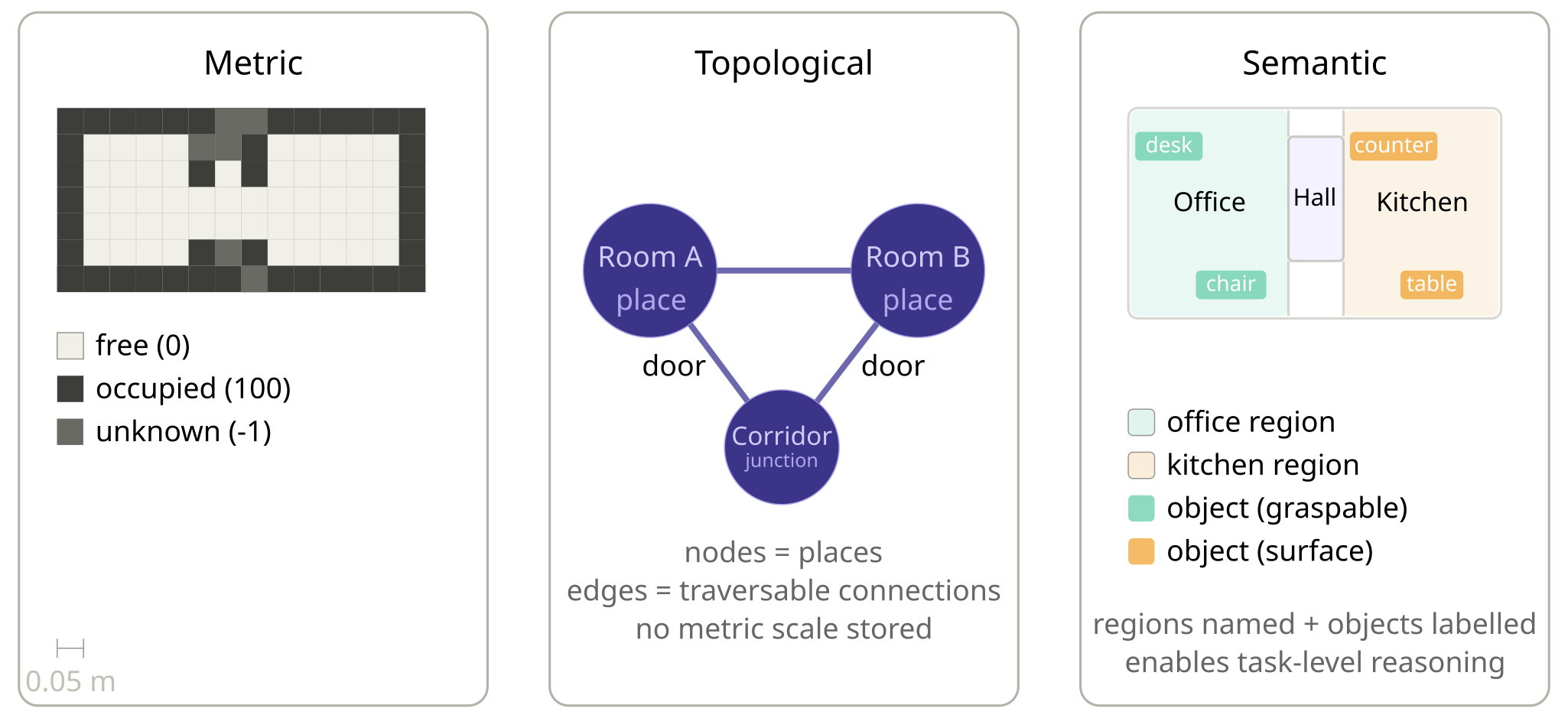
Fig. 100 Map representations: metric, topological, and semantic.

Fig. 101 Map representations: metric, topological, and semantic.

Occupancy Grid Maps

An occupancy grid map is a metric map that divides the environment into a regular grid of cells. Each cell stores a value representing the probability that the corresponding region of space is occupied by an obstacle.

Resources

• nav_msgs/OccupancyGrid message

• REP 105: Coordinate Frames for Mobile Platforms

Grid Parameters

An occupancy grid is defined by a few key parameters:

• Resolution: the width (and height) of one cell in metres. A typical value is 0.05 m (5 cm per cell). Finer resolution gives more detail but requires more memory and computation.

• Width and Height: the number of cells in each dimension. A \(4000 \times 4000\) map at 0.05 m/cell covers a \(200 \times 200\)-m area.

• Origin: the pose of the bottom-left corner of the map in the map frame, stored as a geometry_msgs/Pose.

Note

The nav_msgs/msg/OccupancyGrid message bundles all of this together with the cell data array.

ros2 interface show nav_msgs/msg/OccupancyGrid

Cell States

Each cell in the grid can be in one of three states.

Table 29 Free, occupied, and unknown states

State	Value	Meaning
Free	0	The cell is known to be unoccupied.
Occupied	100	The cell is known to contain an obstacle.
Unknown	-1	The cell has not been observed yet.

Values between 0 and 100 represent intermediate probabilities produced by probabilistic map-update algorithms such as those used by slam_toolbox.

Note

When visualized in RViz2: free cells appear white, occupied cells appear black, and unknown cells appear grey.

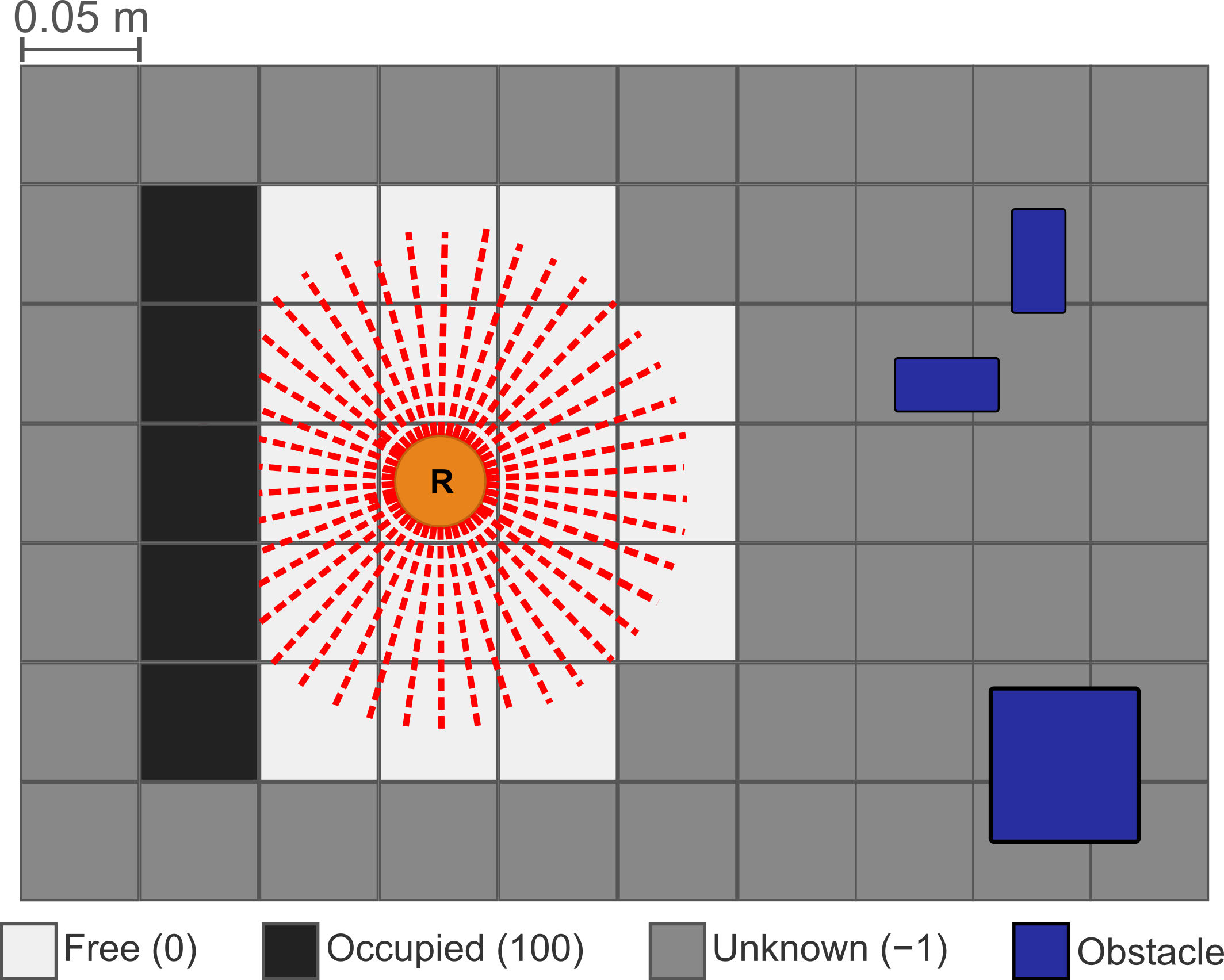
Fig. 102 Occupancy grid: cell states.

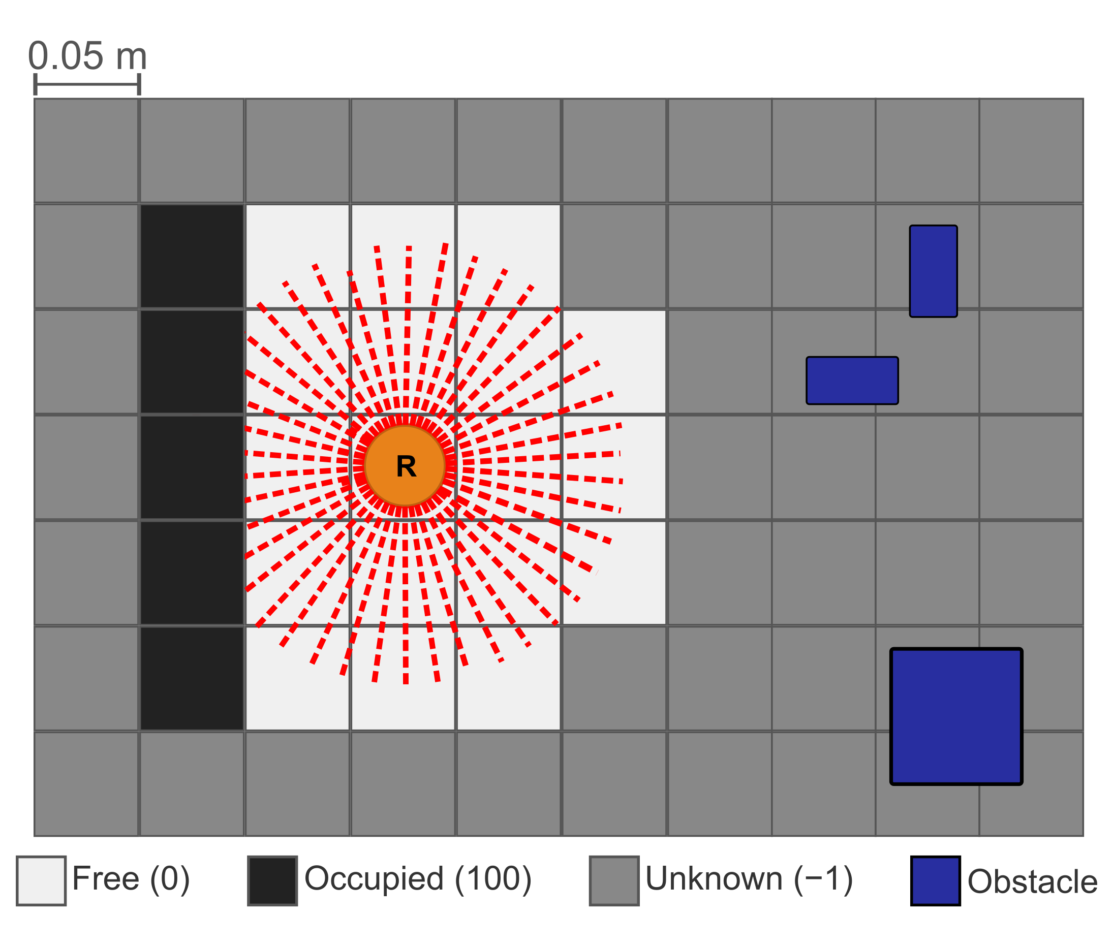
Fig. 103 Occupancy grid: cell states.

Why Probabilities? How LiDAR Updates the Map

Real sensors are noisy: a single reading can be a spurious reflection, a glass surface, or a moving person. A binary free/occupied decision from one scan would be fragile, so probabilistic algorithms accumulate evidence over many scans.

A LiDAR fires many rays per scan. For each ray, slam_toolbox applies a Bayesian update (typically log-odds based) to every cell the ray touches:

• Cells the ray passes through -> probability decreases (evidence for free).

• The cell where the ray terminates -> probability increases (evidence for occupied).

• Cells the ray never reaches -> stay at -1 (unknown).

Example

A cell at the edge of a thin obstacle evolves across four scans (hit, hit, pass-through, hit) as \(65 \rightarrow 80 \rightarrow 70 \rightarrow 85\), stabilizing near \(80\): very likely occupied, with some sensor disagreement.

Note

Downstream consumers (e.g., Nav2 costmaps) apply a threshold to convert probabilities into planning decisions, trading off conservative vs. aggressive behavior.

The map Frame

The map frame is the global reference frame for navigation. REP 105 defines a chain of frames that every mobile robot stack uses.

Table 30 The full REP 105 frame chain

Transform	Who publishes it and why
world \(\to\) map	Published by a higher-level mission system when a global reference is needed. Often omitted in single-robot setups.
map \(\to\) odom	Published by the localization stack (SLAM or AMCL). Corrects accumulated drift by aligning the robot’s estimated pose with the map.
odom \(\to\) base_link	Published by the robot driver (wheel encoders + IMU). Locally consistent; never jumps but drifts over time.
base_link \(\to\) other robot frames	Published by robot_state_publisher from the URDF. Fixed geometric offsets.

Important

The map \(\to\) odom transform can jump when the localization estimate is corrected (e.g., loop closure in SLAM, particle filter convergence in AMCL). This is intentional: the odom frame absorbs smooth motion; the map frame absorbs corrections.

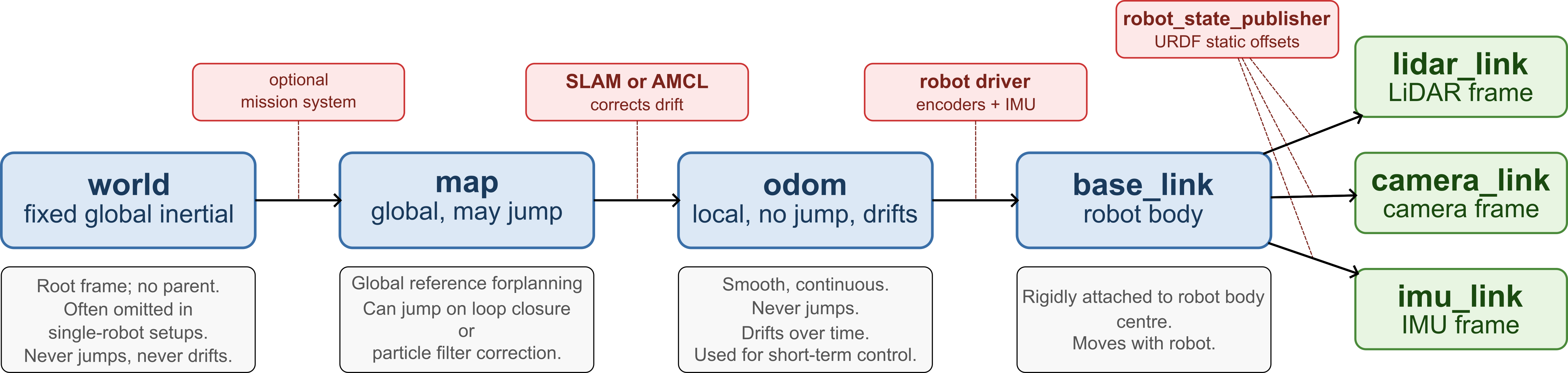
Fig. 104 REP 105 frame chain: who publishes each transform and what it represents.

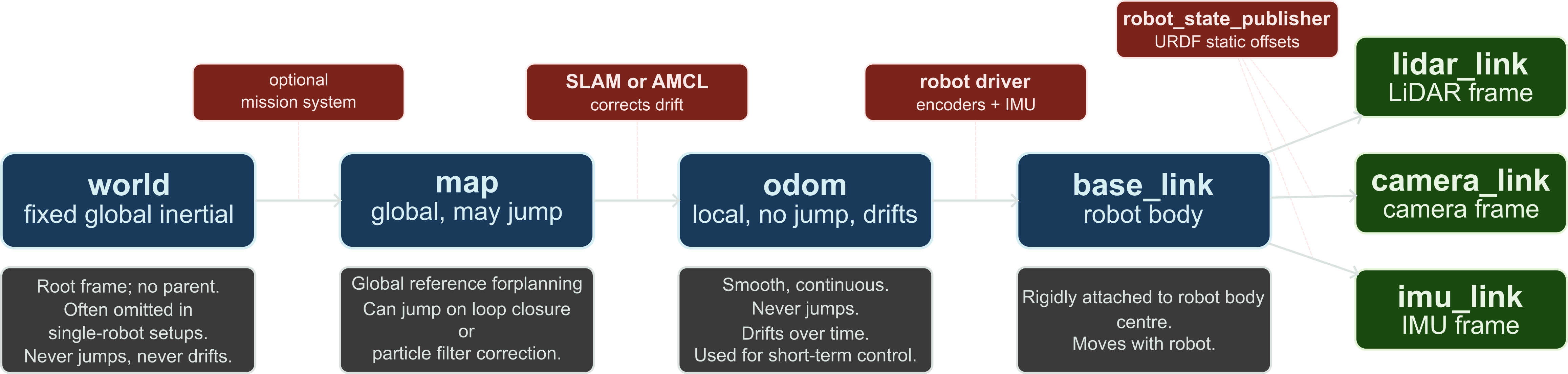
Fig. 105 REP 105 frame chain: who publishes each transform and what it represents.

``map`` vs. ``odom``

	odom	map
Publisher	Robot driver	Localization stack (SLAM/AMCL)
Can jump?	No	Yes (on correction)
Drifts?	Yes (over time)	No (corrected against map)
Use for	Short-term, smooth control	Global planning and goal poses

Note

Navigation goals sent to Nav2 are expressed in the map frame. The planner plans in map. The controller executes in odom. TF2 handles the conversion automatically.

SLAM

SLAM (Simultaneous Localization and Mapping) solves a chicken-and-egg problem: to build a map you need to know where you are, but to know where you are you need a map. SLAM estimates both simultaneously from sensor data alone.

Note

slam_toolbox is a graph-based 2D SLAM library. It builds a pose graph from successive LiDAR scans and corrects accumulated drift through loop closure.

Resources

• Nav2: Using SLAM with slam_toolbox

• slam_toolbox repository

• slam_toolbox ROS 2 documentation

Scan Matching

As the robot moves, the LiDAR produces a stream of scans. Each scan is a snapshot of the surrounding obstacles as seen from the robot’s current position.

• Scan matching aligns two consecutive scans by finding the rigid transformation (translation + rotation) that best overlaps them.

• The result is an estimate of how much the robot moved between the two scans, independently of wheel odometry.

• This incremental pose estimate is much more accurate than wheel odometry alone, especially on slippery or uneven surfaces.

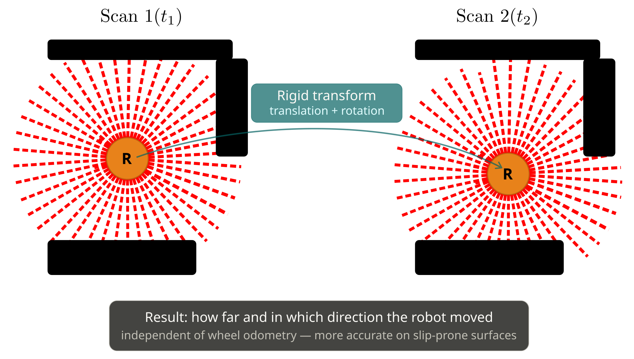
Fig. 106 Scan matching: the LiDAR point cloud from pose \(t_1\) is aligned with the cloud from pose \(t_2\) to recover the rigid transform between them, independently of wheel odometry.

Fig. 107 Scan matching: the LiDAR point cloud from pose \(t_1\) is aligned with the cloud from pose \(t_2\) to recover the rigid transform between them, independently of wheel odometry.

Pose Graph

• Every time the robot moves far enough (configured by minimum_travel_distance and minimum_travel_heading relative to the last node, measured from the incoming odom estimate), slam_toolbox creates a new node representing the robot’s pose at that moment.

• An edge is added between consecutive nodes. Its transform comes from scan matching, not from odometry, so the graph reflects what the LiDAR actually saw.

• The pose graph is a sparse representation of the robot’s trajectory. The occupancy grid is rendered from it by stamping each node’s scan into the grid at the node’s optimized pose.

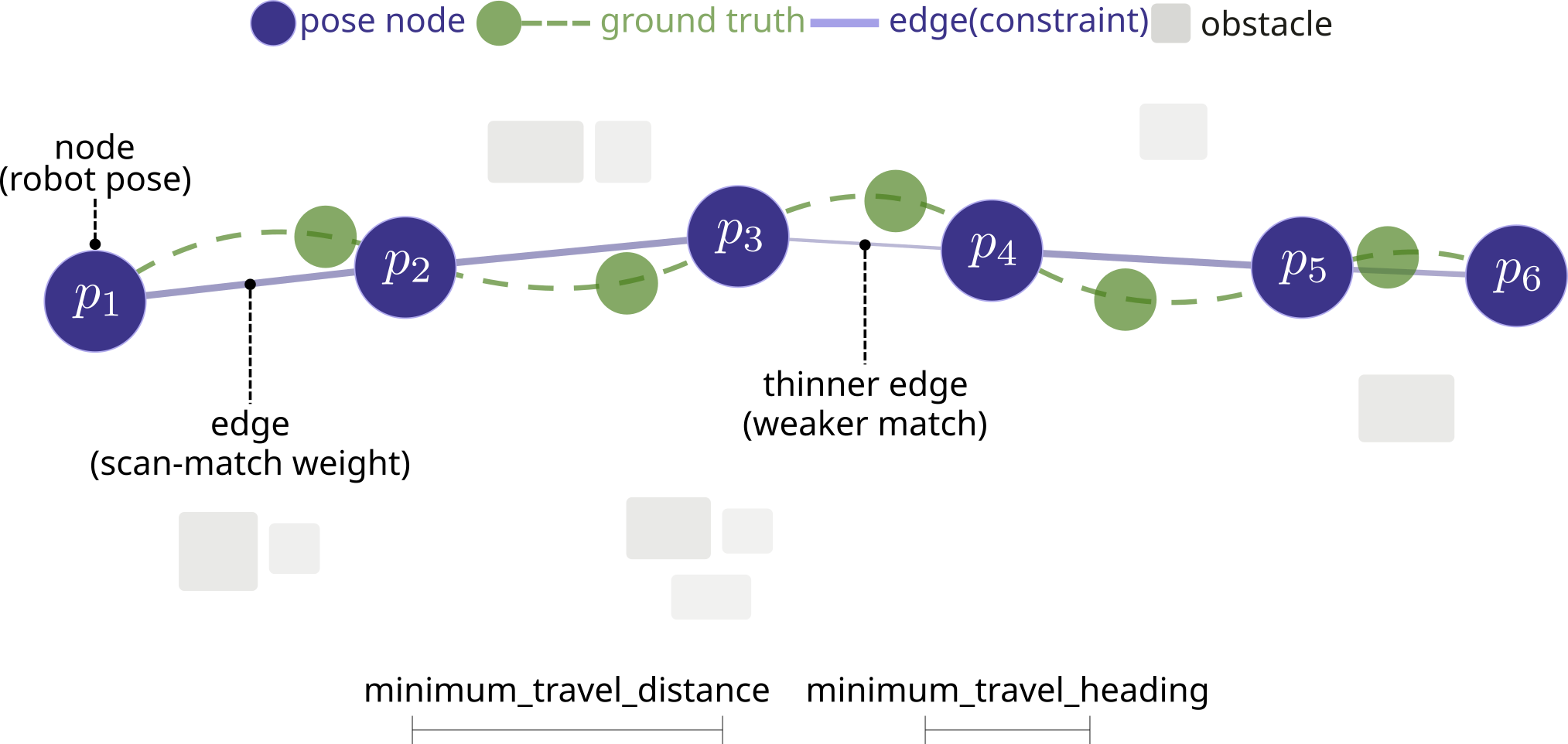
Fig. 108 A pose graph: nodes are estimated robot poses, edges encode the relative transforms between them.

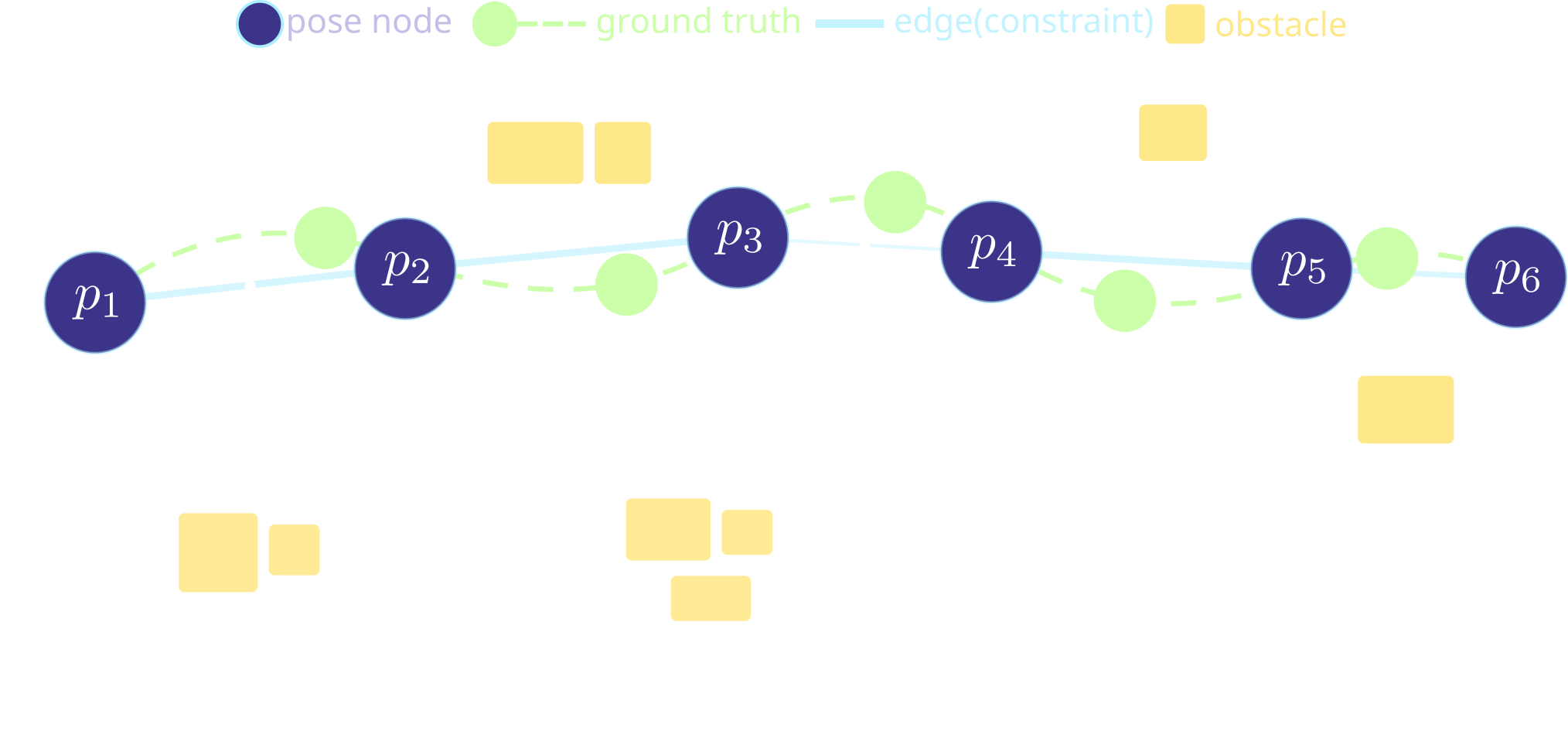
Fig. 109 A pose graph: nodes are estimated robot poses, edges encode the relative transforms between them.

Loop Closure

• When the robot returns near a previously visited area (detected by pose proximity in the graph), the current scan is matched against the stored scan from that earlier visit.

• If the scan match succeeds with high confidence, a loop-closure edge is added connecting the current node to the earlier node.

• The graph is then optimized: all node poses are adjusted to minimize the total inconsistency across odometry edges, scan-match edges, and loop-closure edges. This corrects accumulated drift across the entire trajectory.

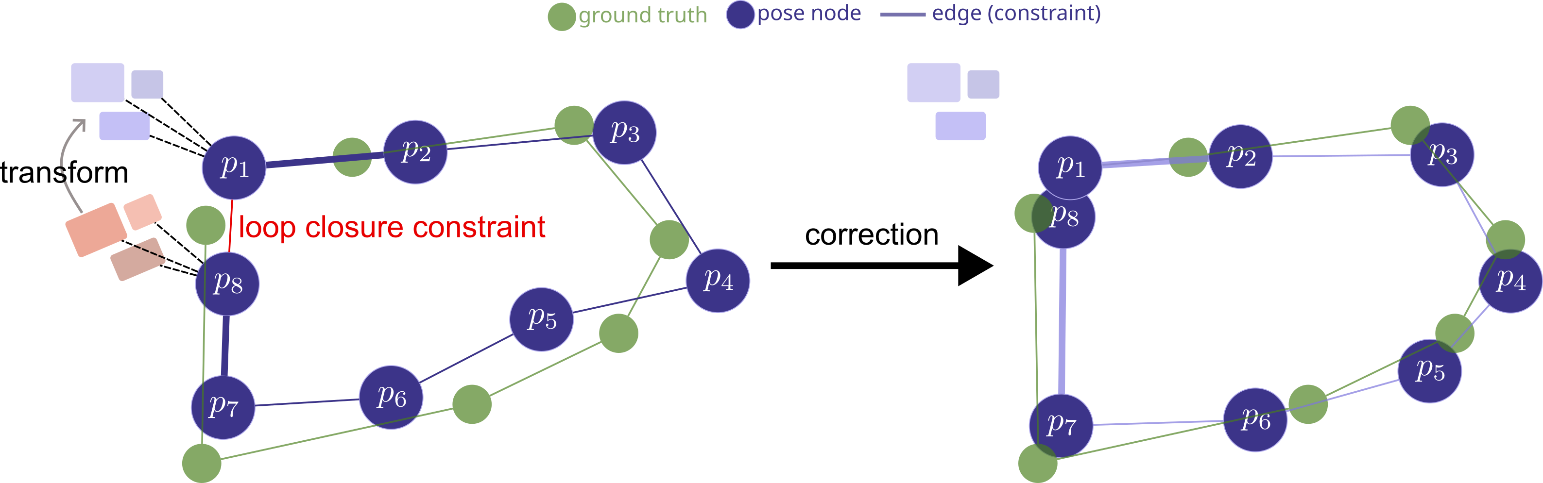
Fig. 110 Loop closure corrects accumulated drift: the loop-closure edge lets graph optimization realign the whole trajectory into a globally consistent map.

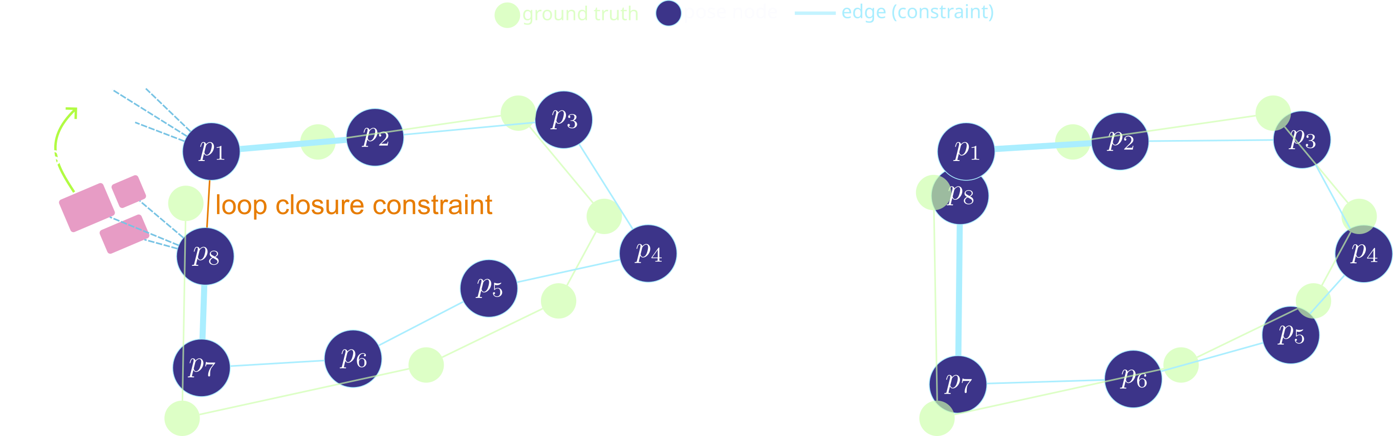
Fig. 111 Loop closure corrects accumulated drift: the loop-closure edge lets graph optimization realign the whole trajectory into a globally consistent map.

Note

Loop closure is why SLAM produces globally consistent maps even after long traversals. Without it, the map would shear and overlap as drift accumulates.

How the Three Pieces Connect

Scan matching, the pose graph, and loop closure form a pipeline:

1. Scan matching produces the edges. It aligns consecutive LiDAR scans to estimate the relative motion (translation + rotation) between two robot poses. Each result becomes a constraint.

   • The covariance (uncertainty) of the scan match result determines the constraint strength. When two scans have many overlapping features and align well, the covariance is small – the optimizer trusts that edge heavily. When scans are sparse or ambiguous (e.g., a featureless corridor), the covariance is large – the optimizer treats that edge as weak and allows other constraints to override it.

2. The pose graph stores the structure. Each pose is a node; each scan-match result is an edge. The graph grows as the robot drives. Sequential edges accumulate drift over time.

3. Loop closure adds correction edges. When the robot revisits a previously seen area, scan matching is performed between the current scan and a stored scan from the earlier visit. This creates a new edge connecting two distant nodes. A graph optimizer then adjusts all node poses simultaneously to minimize the total error, correcting the accumulated drift.

Note

In short: scan matching produces local motion estimates, the pose graph accumulates them, and loop closure constrains the graph globally to fix drift.

Launching slam_toolbox

We launch slam_toolbox alongside Gazebo and RViz2. As the robot moves, the map grows in real time. slam_toolbox is configured via a YAML parameter file. The most important parameters for this course:

Table 31 Key parameters

Parameter	Default	Effect
resolution	0.05	Map cell size in metres.
max_laser_range	20.0	Ignore LiDAR returns beyond this range.
minimum_travel_distance	0.5	Minimum distance before a new node is added.
minimum_travel_heading	0.5	Minimum rotation (rad) before a new node is added.
use_scan_matching	true	Enable scan-to-scan matching.
do_loop_closing	true	Enable loop closure.

Note

The full parameter list is in the slam_toolbox repository under config/mapper_params_online_async.yaml. You rarely need to change parameters beyond resolution and laser range for typical indoor environments.

Demonstration: Building a Map (teleop)

	Command
T1	ros2 launch rosbot_gazebo husarion_world.launch.py rviz:=False
T2	ros2 launch nav_demo map_nav.launch.py mode:=mapping
Gazebo	Drive the robot with teleop
RViz	Observe the map display

Experiment

Drive the robot fast through a narrow corridor. Does the map look accurate? Now drive slowly. What changes? Why does speed affect map quality?

Answer

SLAM quality is bounded by the worst link in the chain of odometry, sensor sweep rate, and scan matching. Speed amplifies all three error sources simultaneously.

The practical rule is: drive at a speed where the displacement between two scans is small compared to the features being mapped, and keep angular velocity especially low since rotational motion distorts LiDAR scans more severely than translation.

Map Saving and Loading

Once a satisfactory map has been built, it is saved to disk and reloaded later for localization-only operation. The nav2_map_server package handles both halves: map_saver_cli writes the grid to disk, and map_server reads the YAML at startup and republishes the grid on /map for AMCL and the costmaps to consume.

Saving the Map

While slam_toolbox is running, save the current map with:

ros2 run nav2_map_server map_saver_cli -f /path/to/husarion_map

This produces two files:

• husarion_map.pgm: a grayscale image where each pixel corresponds to one grid cell. White = free, black = occupied, grey = unknown.

• husarion_map.yaml: metadata file.

image: husarion_map.pgm
mode: trinary
resolution: 0.050
origin: [-11.809, -10.197, 0]
negate: 0
occupied_thresh: 0.65
free_thresh: 0.196

Navigation

Navigation is the capability of a robot to move autonomously from its current pose to a goal pose, while avoiding obstacles and respecting kinematic constraints. The full problem decomposes into several pieces:

• Localization: determining where the robot is on a known map (AMCL).

• Costmap computation: building traversability grids from the map and live sensor data.

• Path planning: computing a collision-free path from start to goal (global planner).

• Path following: issuing velocity commands to track the planned path (local controller).

• Recovery: handling failure modes when planning or control breaks down.

• Orchestration: coordinating all of the above through a behavior tree.

Note

Nav2 is the standard ROS 2 navigation stack and provides all the components needed to do this.

Resources

• Nav2 documentation

• Nav2 concepts overview

The Navigation Problem

Autonomous navigation can be decomposed into four questions, each answered by a different Nav2 component.

Table 32 The four navigation questions

Question	Component	Output
Where am I?	AMCL	Pose estimate in map
What can I traverse?	Costmaps	Cost grid over the environment
How do I get there?	Global planner	Collision-free path to goal
How do I follow the path?	Local controller	Velocity commands on /cmd_vel

Note

SLAM answers a fifth question that precedes all of the above: what does the environment look like? Once the map is built and saved, Nav2 takes over and the robot can navigate indefinitely on that map.

Demonstration: End-to-End Nav2

	Command
T1	ros2 launch rosbot_gazebo husarion_world.launch.py rviz:=False use_sim:=True
T2	ros2 launch nav_demo map_nav.launch.py mode:=navigation
RViz	Click 2D Pose Estimate and set the initial pose
RViz	Click Nav2 Goal and click somewhere in the map

Localization

Localization is the process of determining the robot’s pose within a known map. Wheel odometry alone drifts over time, so the robot must continuously correct its estimated pose by matching sensor observations (typically LiDAR) against the map.

Resources

• Nav2: Configuring AMCL

• nav2_amcl documentation

AMCL (Adaptive Monte Carlo Localization)

AMCL maintains a probability distribution over possible robot poses, represented as a cloud of particles, and continuously refines it using LiDAR data.

Why “Adaptive”?

Standard MCL uses a fixed number of particles regardless of how certain the filter is. AMCL adapts:

• When the particle cloud is widely spread (robot is lost), more particles are used to cover the uncertainty.

• When the particle cloud has converged (robot is well-localized), fewer particles are needed, reducing CPU cost.

Launching AMCL

AMCL requires a running map_server and an initial pose estimate. Once given those, it publishes the map \(\to\) odom transform continuously.

Setting the Initial Pose

AMCL needs a starting guess for the robot’s pose. Without it, particles are spread uniformly over the whole map and convergence is slow.

Three ways to provide the initial pose:

• RViz2: click the 2D Pose Estimate button in the toolbar, then click and drag on the map to set the position and orientation. AMCL receives a geometry_msgs/msg/PoseWithCovarianceStamped message on /initialpose.

• Parameter: set set_initial_pose: true in the AMCL config and provide initial_pose_x, initial_pose_y, initial_pose_a (yaw). Useful for scripted testing.

• Programmatically with setInitialPose() from BasicNavigator.

Important

A poor initial pose estimate does not prevent localization, but convergence will be slower and the robot may temporarily follow an incorrect path. Always set the initial pose as accurately as possible when starting AMCL.

SLAM vs. AMCL

SLAM and AMCL both produce the map \(\to\) odom transform. Choosing between them depends on whether you already have a map.

Table 33 SLAM vs. AMCL

	SLAM	AMCL
Requires a prior map?	No (builds one from scratch)	Yes (needs a saved map)
Map output?	Yes (produces /map)	No (consumes /map)
Pose estimate?	Yes	Yes
When to use	First deployment, new environment	Known environment, deployment phase
Typical workflow	Drive around to build map, save it	Load map, set initial pose, navigate

Note

slam_toolbox also has a localization mode: it loads an existing map and localizes against it without adding new data, similar to AMCL. This is useful when you trust the map completely and want to avoid modifying it during operation.

Particle Filters

A particle filter represents the robot’s pose distribution as a set of weighted hypotheses. Each hypothesis is a candidate pose \((x, y, \theta)\); its weight reflects how well the sensor data matches the map at that pose.

Particles as Pose Hypotheses

Each particle is an independent guess about where the robot is on the map: a pose \((x, y, \theta)\) with an associated weight. At startup, particles are spread across the map, or across a region near an initial pose estimate if one is provided.

Scoring a Particle

To decide how good a guess is, AMCL asks: if the robot were really at this pose, what would the LiDAR see?

1. Place a virtual LiDAR at the particle’s pose \((x, y, \theta)\) on the map.

2. For each beam of that virtual LiDAR, cast a ray into the map until it hits an occupied cell. The distance to that cell is the predicted range.

3. Compare the predicted range to the actual range measured by the real LiDAR on the robot.

4. If the predicted and actual ranges agree across most beams, the particle is probably near the true pose and its weight goes up. If they disagree, the weight goes down.

Note

A particle correctly placed in the hallway predicts walls at roughly the distances the real LiDAR measures. A particle wrongly placed inside a room predicts walls much closer or farther than what the LiDAR actually sees, and is penalized.

The Particle Filter Cycle

AMCL repeats three steps every time new odometry and a new LiDAR scan arrive:

1. Predict: shift every particle by the robot’s measured motion, plus a small amount of noise (the motion model). Particles spread out slightly to reflect uncertainty in the motion.

2. Update: score each particle by comparing its predicted LiDAR scan against the actual scan. Well-matching particles get higher weights.

3. Resample: draw a new set of particles with replacement, proportional to weights. High-weight particles are likely duplicated; low-weight particles are likely dropped.

What Happens Over Time

Early on, particles are scattered and weights are mixed. After a few cycles of motion and observation, the particle cloud concentrates around poses that consistently explain the LiDAR data. The robot’s estimated pose is then reported as a summary of this cloud (typically the weighted mean).

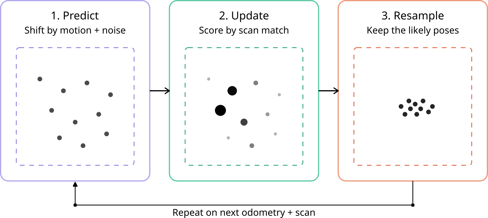
Fig. 112 AMCL predict/update/resample cycle. Particle size encodes weight; after resampling, particles concentrate near the true pose.

Fig. 113 AMCL predict/update/resample cycle. Particle size encodes weight; after resampling, particles concentrate near the true pose.

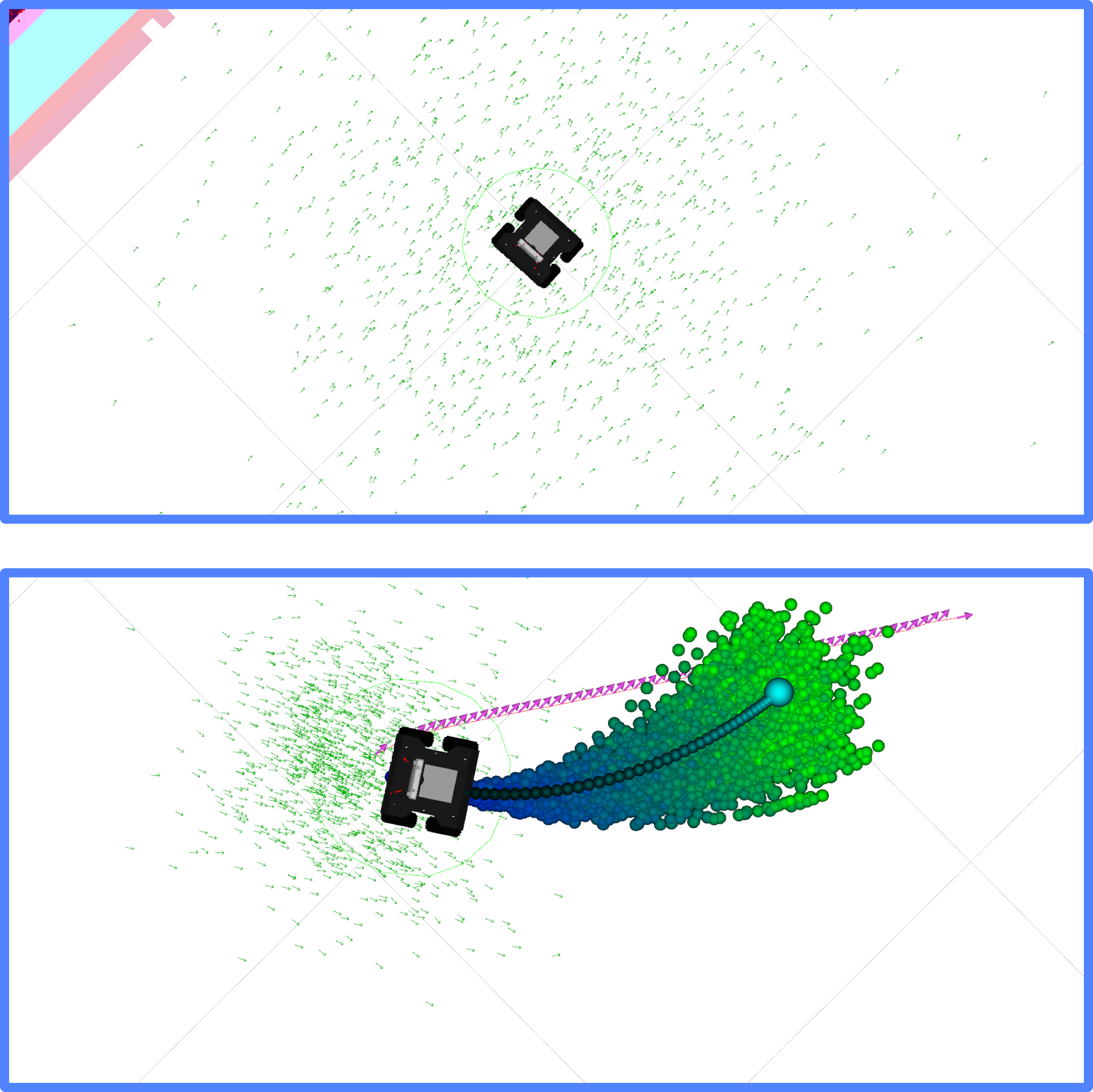
Fig. 114 Particle filters at initialization (top) and when the robot is driving towards a goal (bottom).

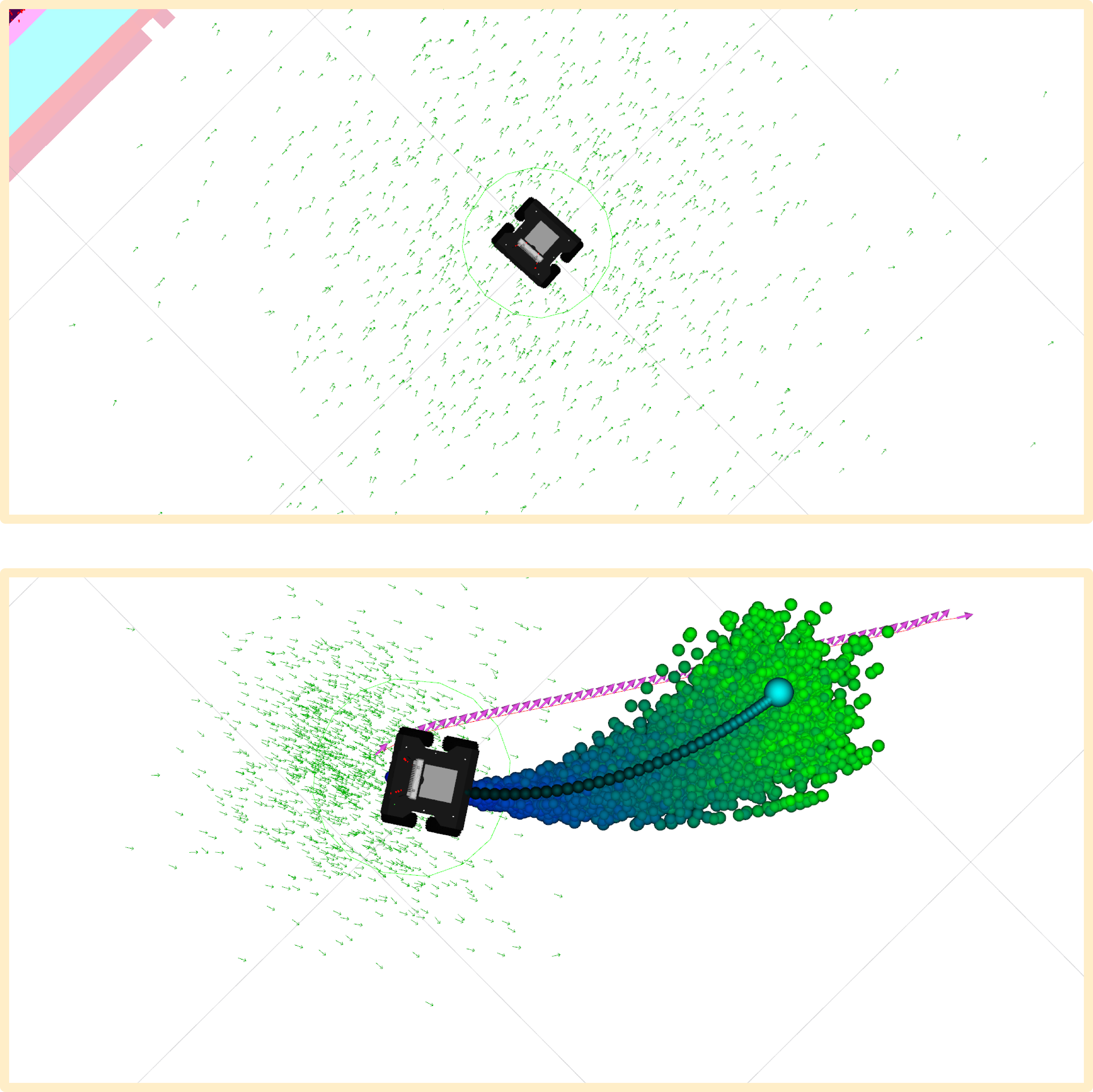
Fig. 115 Particle filters at initialization (top) and when the robot is driving towards a goal (bottom).

Costmaps

A costmap assigns a traversal cost to every cell of a grid. A cost of zero means the cell is freely traversable; a lethal cost means the robot’s footprint would collide with an obstacle if the robot centre were placed there.

Resources

• Nav2: Configuring Costmaps

• Nav2 Concepts: Costmaps

Global vs. Local Costmap

Nav2 maintains two costmaps. The global costmap covers the entire map and is used by the planner. The local costmap covers a rolling window around the robot and is used by the controller.

Table 34 Comparison of the global and local costmaps in Nav2

	Global Costmap	Local Costmap
Extent	Full map	Rolling window around robot (e.g., \(5 \times 5\) m)
Used by	Global planner	Local controller
Update rate	Slower	Faster (matches sensor rate)
Handles dynamic obstacles?	No (static map only)	Yes (live sensor data)
Published on	/global_costmap/costmap	/local_costmap/costmap

Note

The global costmap is responsible for finding a collision-free path from start to goal. The local costmap handles obstacles that appear while the robot is moving, such as a person walking into the corridor.

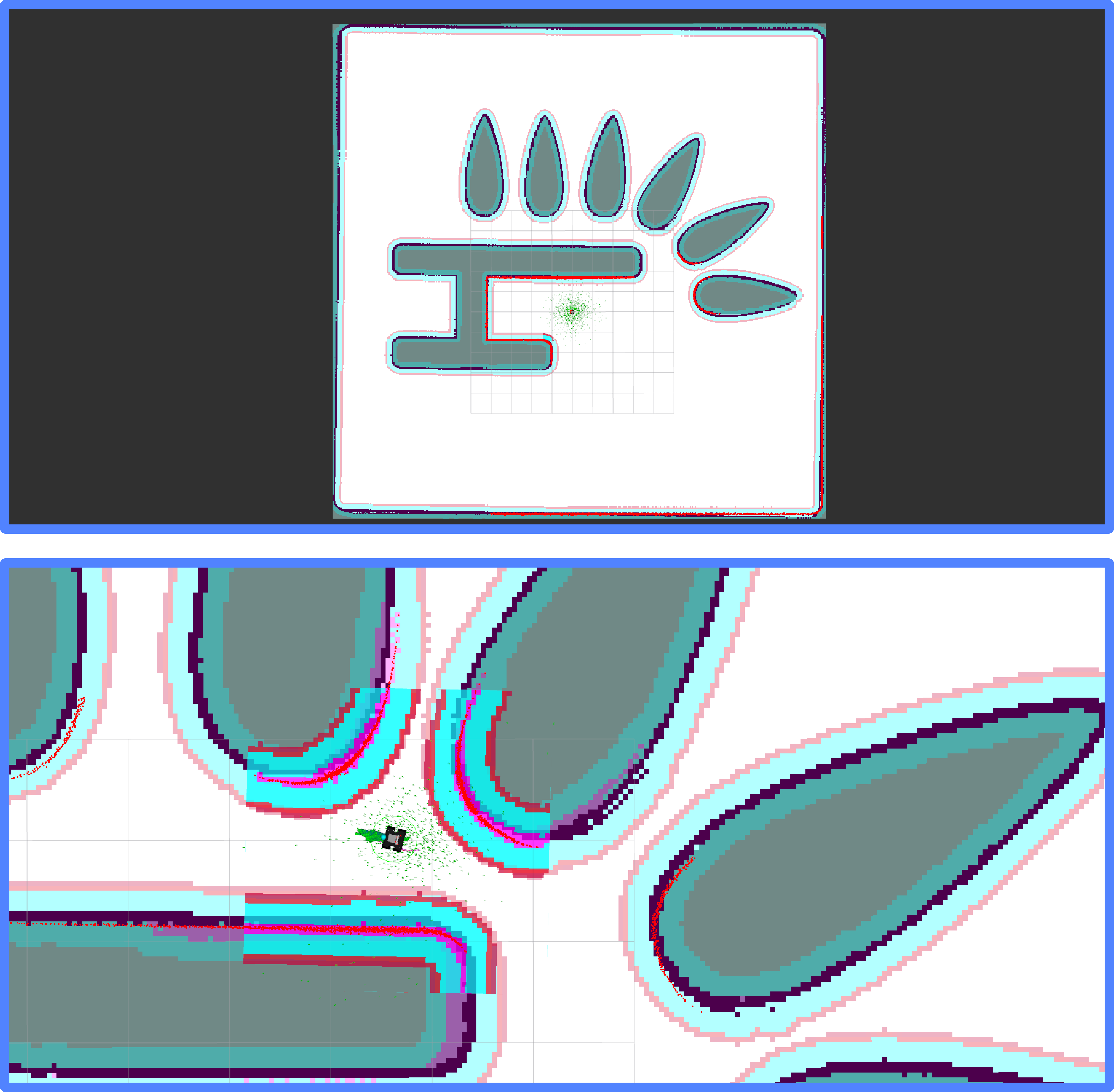
Fig. 116 Global and local costmaps.

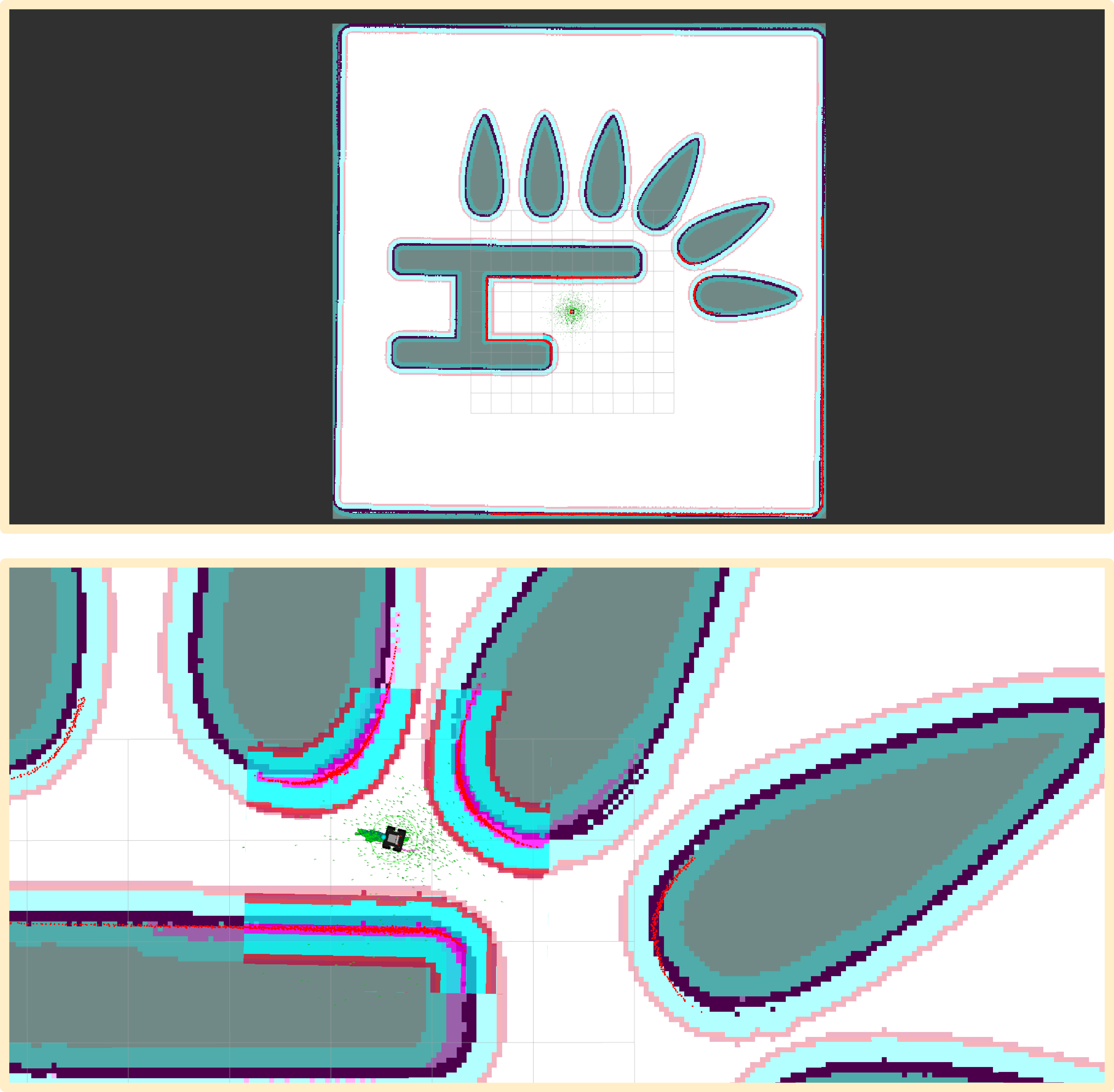
Fig. 117 Global and local costmaps.

Costmap Layers

Each costmap is composed of stacked layers, each contributing to the final cost grid:

• Static layer: reads the /map topic and marks occupied cells as lethal. Present in the global costmap; optional in the local costmap.

• Obstacle layer: reads live sensor data (LiDAR, depth camera) and marks newly observed obstacles. Present in both costmaps. Obstacles decay over time if not re-observed.

• Inflation layer: expands lethal cells outward by a configurable radius. Cells close to obstacles get elevated (but non-lethal) cost, creating a gradient that steers the robot away from walls.

Note

The inflation radius should be at least as large as the robot’s circumscribed radius. A larger inflation radius gives safer paths at the cost of narrower passable corridors.

Robot Footprint

The footprint is the 2D polygon representing the robot’s outline in the base_link frame. Nav2 uses it – together with the costmap – to decide which cells are lethal: a cell is lethal if placing the footprint there would overlap an obstacle.

• Inscribed radius (\(r_i\)): the largest circle that fits inside the footprint. A cell at distance \(< r_i\) from an obstacle is always lethal regardless of orientation.

• Circumscribed radius (\(r_c\)): the smallest circle that encloses the footprint. A cell at distance \(> r_c\) is always safe regardless of orientation.

• Between \(r_i\) and \(r_c\), safety depends on the robot’s heading.

Note

For a robot modeled as a circle, \(r_i = r_c\), so orientation no longer affects collision checking. This is why many differential-drive robots use a circular footprint even when the chassis is rectangular: it trades a small loss in fidelity for a much simpler planning problem.

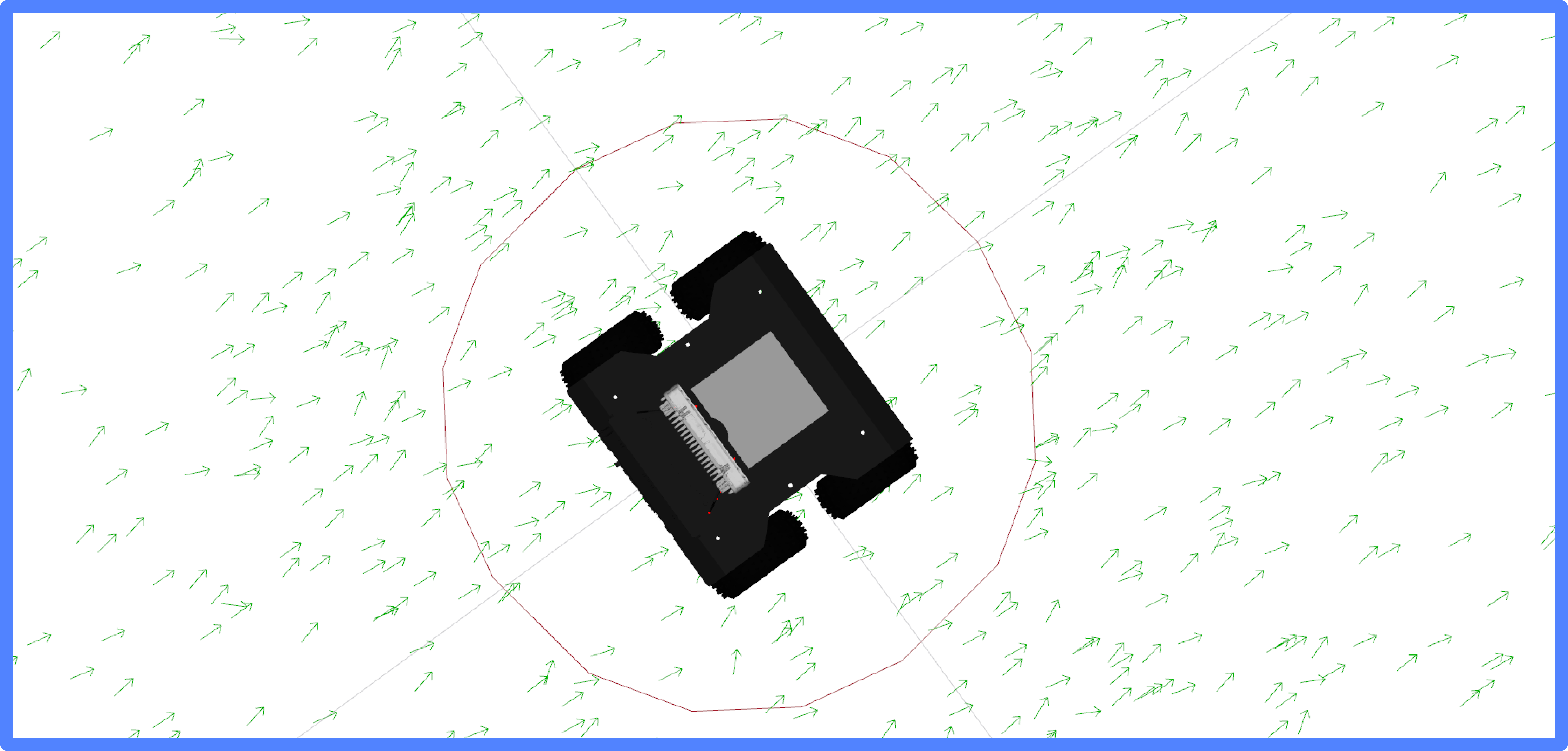
Fig. 118 Robot’s footprint (red polygon).

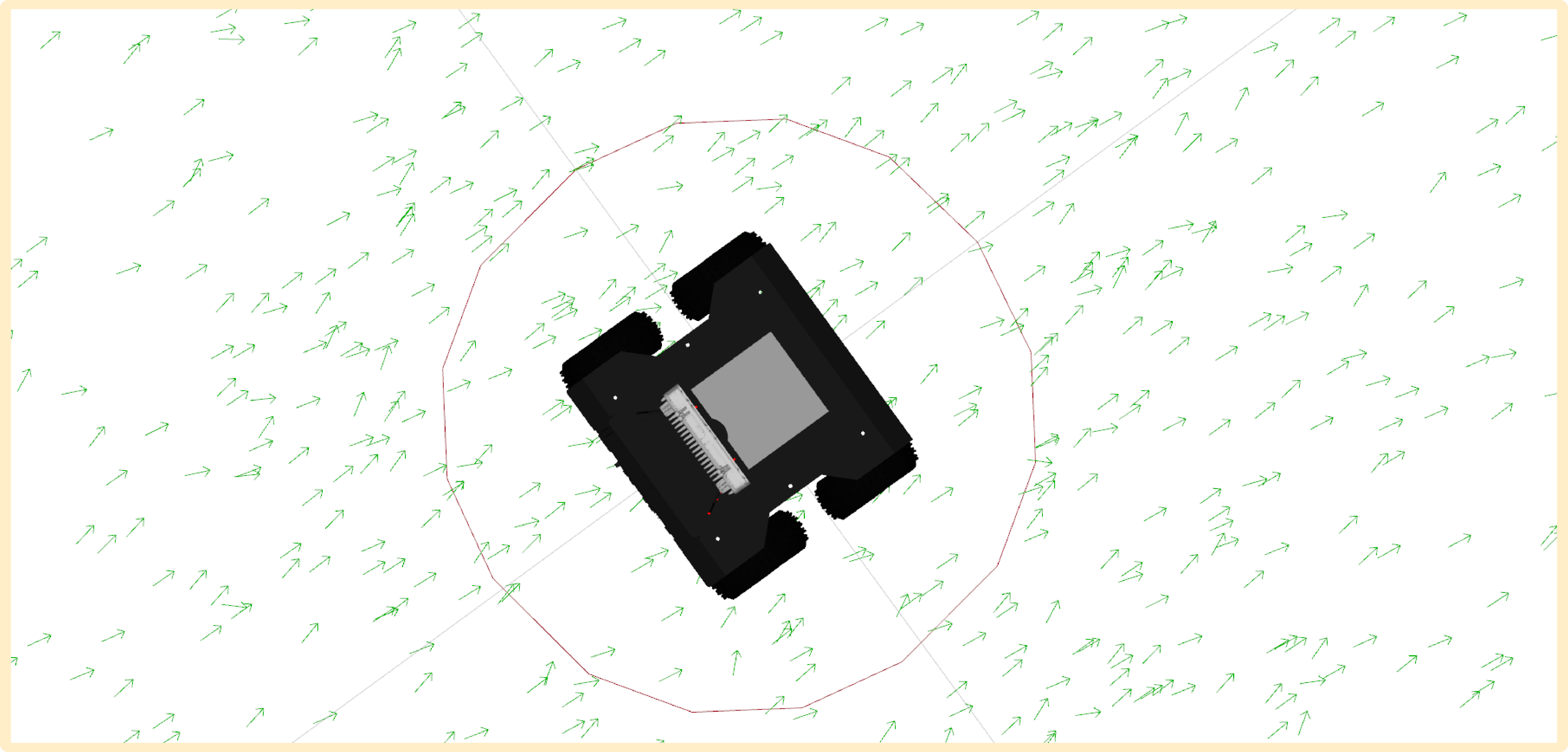
Fig. 119 Robot’s footprint (red polygon).

Planning and Control

Nav2 separates navigation into two distinct problems: planning (find a collision-free path from start to goal) and control (follow that path while avoiding dynamic obstacles). Each problem has dedicated plugins.

Resources

• Nav2: NavFn Planner

• Nav2: Smac Planner

• Nav2: DWB Controller

• Nav2: Regulated Pure Pursuit

Global Planners

A global planner computes a path from the robot’s current pose to the goal pose using the global costmap. The path is a sequence of poses expressed in the map frame.

Table 35 Global planners available in Nav2

Planner	Algorithm	When to prefer it
NavFn	Dijkstra or A* on a grid	Simple environments, fast replanning, does not enforce kinematic constraints.
Smac Hybrid A*	Kinematically constrained A* (SE2 lattice)	Non-holonomic robots, tight spaces, when the path must be physically drivable from the start.
Theta*	Any-angle A* (part of Smac)	Reduces unnecessary turns on open terrain.

• The planner outputs a nav_msgs/msg/Path: a list of geometry_msgs/msg/PoseStamped waypoints.

• The path is published on /plan and visible in RViz2 as a green line.

• The planner is called once per goal request (and replanned if the path becomes blocked).

• Multiple planners can be loaded simultaneously, but only one is used per planning request. The behavior tree selects the planner by name.

Local Controllers

A local controller takes the global path and the local costmap and computes a velocity command for the robot at every control cycle. It runs continuously while the robot is moving.

Table 36 Local controllers available in Nav2

Controller	Approach	When to prefer it
DWB	Samples candidate velocities and picks the best one.	Crowded dynamic environments; tunable scoring weights.
Regulated Pure Pursuit (RPP)	Follows the path toward a lookahead point, slowing near obstacles and curves.	Open environments, smooth paths, when computational cost matters.

• Both controllers publish geometry_msgs/msg/TwistStamped on /cmd_vel.

• The controller runs at a configurable rate (typically 20 Hz).

• If the controller cannot find a valid command (e.g., path is blocked), it reports failure and the behavior tree triggers a recovery behavior.

• Multiple controllers can be loaded simultaneously, but only one runs per control cycle. The behavior tree selects the controller by name.

Behavior Trees and Recovery

Nav2 orchestrates planning, control, and recovery through a behavior tree (BT). Rather than a fixed sequence of steps, a BT allows flexible, modular composition of navigation behaviors with built-in error handling.

Recovery Behaviors in Nav2

When the planner or controller fails, the BT falls back to recovery behaviors:

• Spin: rotate in place to get unstuck.

• Wait: pause and wait for a blocked path to clear.

• Clear costmap: erase the local costmap to remove stale obstacle markings.

• Back up: drive a short distance in reverse.

Resources

• Nav2: Behavior Trees

• BehaviorTree.CPP documentation

NavigateToPose Action API

NavigateToPose is the primary ROS 2 action interface for the Nav2 stack. A client sends a goal pose; Nav2 plans, controls, and recovers autonomously until the robot reaches the goal or fails.

Resources

• Nav2 Simple Commander API

• nav2_msgs/action/NavigateToPose interface

Goal / Feedback / Result

• Goal: sent once by the client to initiate the task. For NavigateToPose, the goal is a geometry_msgs/msg/PoseStamped in the map frame.

• Feedback: published periodically by the server while the task is running. For NavigateToPose, feedback includes the current pose, time elapsed, distance remaining, and the number of recoveries attempted.

• Result: sent once when the task completes (success or failure). For NavigateToPose, the result is empty; success or failure is conveyed by the goal status code.

ros2 interface show nav2_msgs/action/NavigateToPose

Note

Actions can also be preempted: a client can cancel a goal mid-execution. Nav2 will stop the robot cleanly and report the goal as cancelled.

Sending a Goal in RViz

RViz2 provides the simplest way to send a navigation goal: the Nav2 Goal button. Clicking it lets you pick a pose on the map; RViz publishes it on /goal_pose, which the BT Navigator converts into a NavigateToPose action goal.

Note

This is the fastest way to verify that the full stack – planner, controller, and recoveries – is working end to end before writing any client code.

Demonstration: Send a Goal from RViz

	Command
T1	ros2 launch rosbot_gazebo husarion_world.launch.py rviz:=False use_sim:=True
T2	ros2 launch nav_demo map_nav.launch.py mode:=navigation
RViz	Click 2D Pose Estimate
RViz	Click Nav2 Goal and click somewhere in the map

Sending a Goal Programmatically

The Python way to send goals is to use the NavigateToPose action client. Nav2 ships nav2_simple_commander, a high-level wrapper that handles the boilerplate – creating the client, waiting for the server, sending goals, and tracking feedback.

Simple Commander

The nav2_simple_commander package provides BasicNavigator, a high-level Python API that wraps the Nav2 action interfaces. It handles action client creation, initial pose setting, and goal management in a few method calls.

Resources

• Nav2 Simple Commander API

• nav2_simple_commander source

BasicNavigator: Key Methods

Table 37 Key methods of BasicNavigator

Method	Description
setInitialPose(pose)	Send an initial pose estimate to AMCL.
waitUntilNav2Active()	Block until all Nav2 lifecycle nodes are active.
goToPose(pose)	Send a single NavigateToPose goal.
followWaypoints(poses)	Send a list of waypoints to the waypoint follower.
isTaskComplete()	Returns True when the current task finishes.
getFeedback()	Returns the latest feedback from the active task.
getResult()	Returns the TaskResult enum (SUCCEEDED, CANCELED, FAILED).
cancelTask()	Cancel the current goal.

Note

BasicNavigator creates its own ROS 2 node internally; you do not need to pass it a node reference – just instantiate it and call methods.

Example #1: Navigate to a Single Goal

1. Create a BasicNavigator

self._navigator = BasicNavigator()

2. Set the initial pose from the map \(\to\) base_link TF

self._initial_pose = PoseStamped()
self._initial_pose.header.frame_id = "map"
self._initial_pose.header.stamp = self._navigator.get_clock().now().to_msg()
try:
    tf = self._tf_buffer.lookup_transform(
        "map", "base_link", rclpy.time.Time(),
        timeout=rclpy.duration.Duration(seconds=2.0),
    )
    self._initial_pose.pose.position.x = tf.transform.translation.x
    self._initial_pose.pose.position.y = tf.transform.translation.y
    self._initial_pose.pose.position.z = tf.transform.translation.z
    self._initial_pose.pose.orientation = tf.transform.rotation
except Exception:
    self.get_logger().info("map->base_link TF not available yet.")

self._navigator.setInitialPose(self._initial_pose)

3. Build the goal pose

goal = self.create_pose_stamped(x, y, 0.0)

4. Send it to Nav2

self._navigator.goToPose(goal)

Demonstration: Single Goal

	Command
T1	ros2 launch rosbot_gazebo husarion_world.launch.py rviz:=False
T2	ros2 launch nav_demo map_nav.launch.py mode:=navigation goal_source:=single_goal

Example #2: Follow Waypoints

def follow_waypoints(self):
    self._navigator.waitUntilNav2Active()  # Wait for the Nav2 stack

    pose1 = self.create_pose_stamped(2.0, 0.0, 0.0)
    pose2 = self.create_pose_stamped(5.0, 1.0, 1.57)
    pose3 = self.create_pose_stamped(-5.42, 11.22, 3.14)
    waypoints = [pose1, pose2, pose3]
    self._navigator.followWaypoints(waypoints)

Note

See nav_demo/navigation_demo_interface.py for the complete example: it sets the initial pose from TF and handles feedback and results.

Demonstration: Follow Waypoints

	Command
T1	ros2 launch rosbot_gazebo husarion_world.launch.py rviz:=False
T2	ros2 launch nav_demo map_nav.launch.py mode:=navigation goal_source:=waypoints

Explore Mode: Map and Navigate Simultaneously

When mode:=explore is selected, two groups activate. The SLAM group includes online_async_launch.py from slam_toolbox, which subscribes to the LiDAR and publishes a continuously updated nav_msgs/OccupancyGrid on /map. The Nav2 group includes navigation_launch.py from nav2_bringup, which consumes that same /map topic to build its global costmap. AMCL is not started, because slam_toolbox is already publishing the map \(\to\) odom transform itself.

Demonstration: Explore Mode

	Command
T1	ros2 launch rosbot_gazebo husarion_world.launch.py rviz:=False
T2	ros2 launch nav_demo map_nav.launch.py mode:=explore goal_source:=manual

Note

In explore mode, the map and the plan evolve together. As the robot drives into unknown space, slam_toolbox extends the occupancy grid, the costmap inflates around new obstacles, and the global planner immediately re-routes around them. This is what enables true autonomous exploration of unmapped environments.